Understanding Loss and Cost Functions
To find the optimal parameters (like w and b) for a model, we first need a way to measure how well the model is performing. We do this with loss and cost functions.
- A Loss Function measures the error for a single training example.
- A Cost Function is the average of the loss over the entire training dataset.
The goal of training is to find the parameters that minimize the cost function.
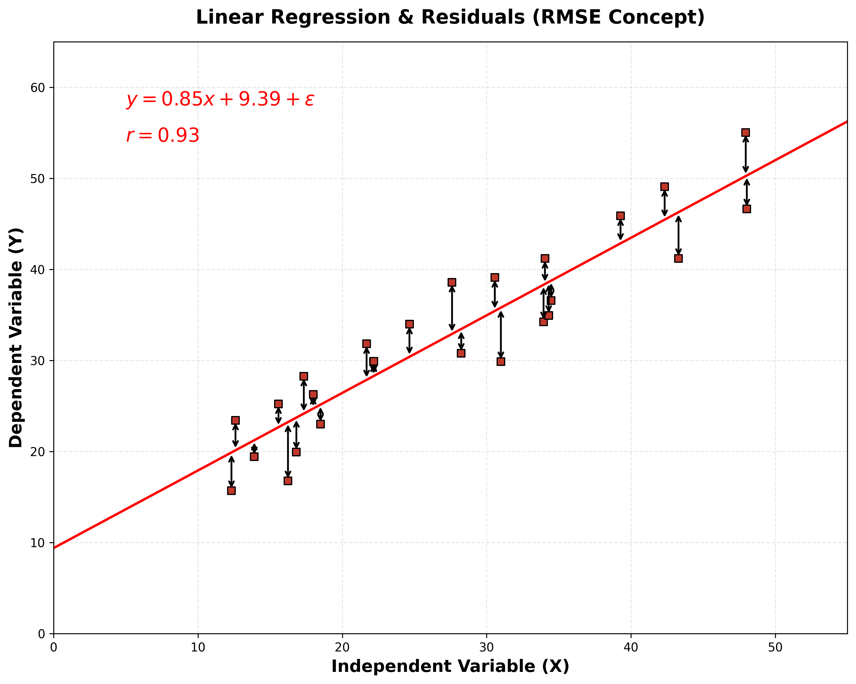
For Linear Regression: Mean Squared Error (MSE)
For a single training example in linear regression, the loss is the squared error:
Loss = (ŷ - y)²
where ŷ is the predicted value and y is the actual value.
The cost function is the average of these squared errors over all m examples in the dataset. This is called the Mean Squared Error (MSE).
Cost (MSE) = (1/m) * Σ(ŷᵢ - yᵢ)²
To bring the error back to the original units of the target variable, we often take the square root of the MSE, which gives us the Root Mean Squared Error (RMSE). RMSE is the standard deviation of the prediction errors (residuals) and is a popular metric for evaluating regression models.
Here is an example of calculating RMSE using scikit-learn:
from sklearn.metrics import mean_squared_error
import numpy as np

y_train = [0.5, 0, 0.6, 0.8, 1, 0.8, 0.9]
y_pred = [0.6, 0, 0.6, 0.9, 0.9, 0.7, 0.9]

mse = mean_squared_error(y_train, y_pred)
rmse = np.sqrt(mse)
print(f"RMSE: {rmse}")
Evaluating Regression Models: R-squared (R²)
While RMSE tells us the average error, R-squared (R²), or the coefficient of determination, tells us what proportion of the variance in the target variable is explained by our model's features.
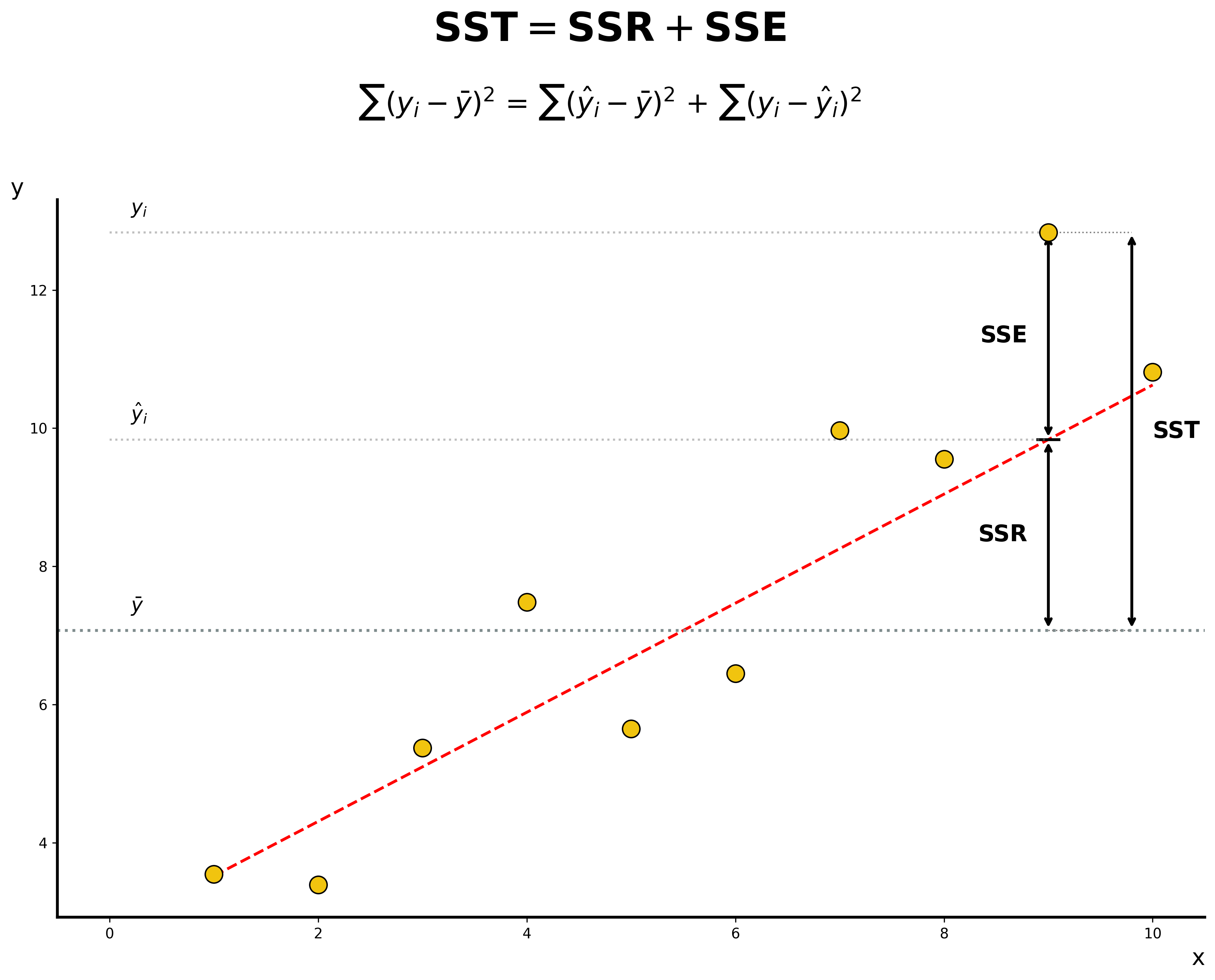
R² is calculated using three components:
- Sum of Squares Total (SST): The total variability in the data.
Σ(yᵢ - y_mean)² - Sum of Squared Regression (SSR): The variability explained by the model.
Σ(ŷᵢ - y_mean)² - Sum of Squared Error (SSE): The unexplained variability (the error).
Σ(yᵢ - ŷᵢ)²
The relationship is: SST = SSR + SSE
R² is the ratio of explained variability to total variability:
R² = SSR / SST = 1 - (SSE / SST)
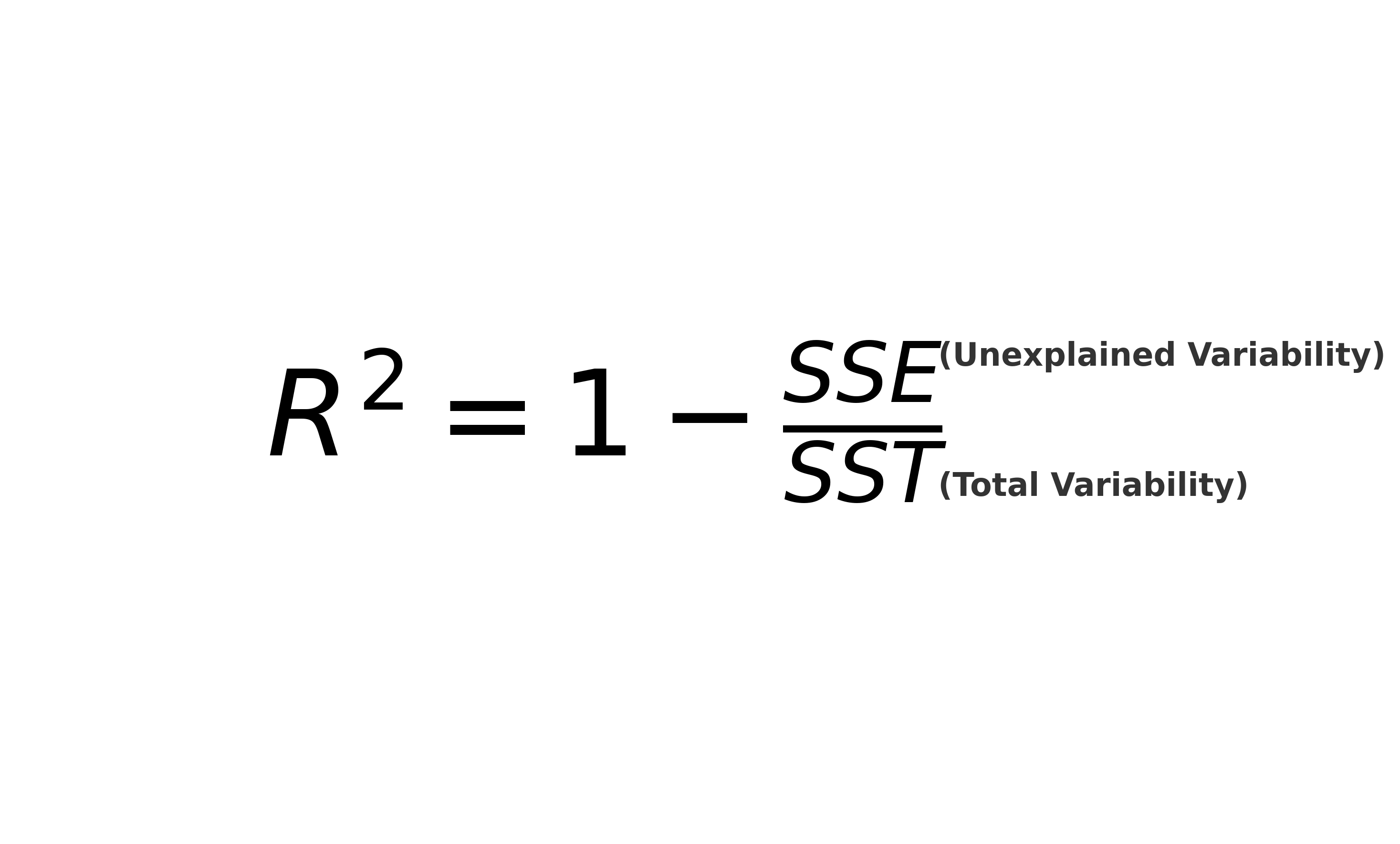
R² ranges from 0 to 1. An R² of 0 means the model explains none of the variability, while an R² of 1 means it explains all of it.
Note on Adjusted R²: A limitation of R² is that it always increases as you add more features, even if they are not useful. Adjusted R² is a modified version that penalizes the score for adding non-significant features, making it a more reliable metric when comparing models with different numbers of features.
For Logistic Regression: Log Loss (Binary Cross-Entropy)
MSE is not a suitable cost function for logistic regression because the sigmoid function would make the cost landscape non-convex (full of local minima). Instead, we use a cost function called Log Loss (or Binary Cross-Entropy).
The loss for a single example is:
Loss = -[y*log(ŷ) + (1-y)*log(1-ŷ)]
This function penalizes the model heavily when it makes a confident prediction that is wrong. The cost function is the average of this loss over the entire dataset.
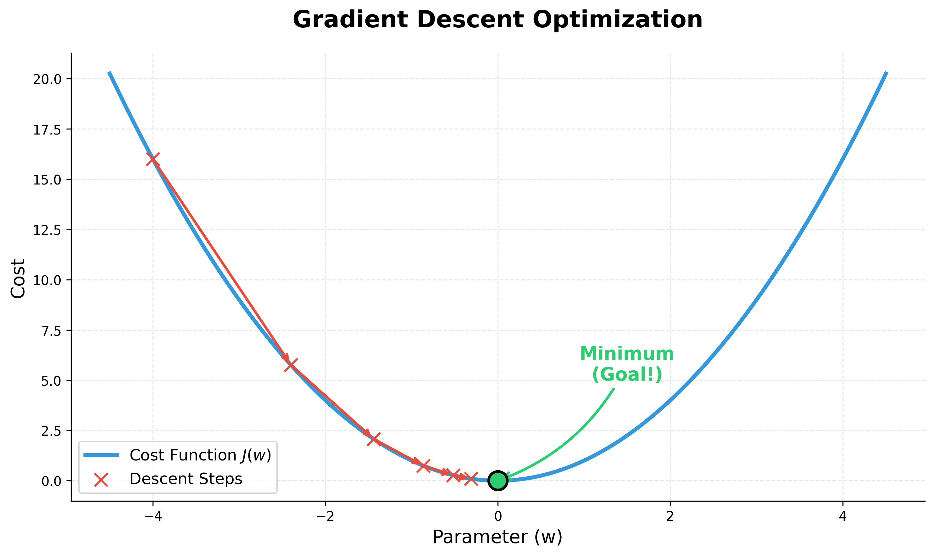
How to Minimize the Cost Function: Gradient Descent
Now that we have a cost function, how do we find the values of w and b that minimize it? While OLS provides a direct formula for linear regression, a more general and widely used optimization algorithm is Gradient Descent.
The intuition is simple: imagine the cost function creates a landscape with hills and valleys. We want to find the lowest point in a valley. Gradient Descent does this by:
- Starting at a random point (random
wandb). - Calculating the slope (gradient) at that point.
- Taking a small step downhill in the direction of the negative gradient.
- Repeating this process until it converges at the bottom of the valley (the minimum cost).
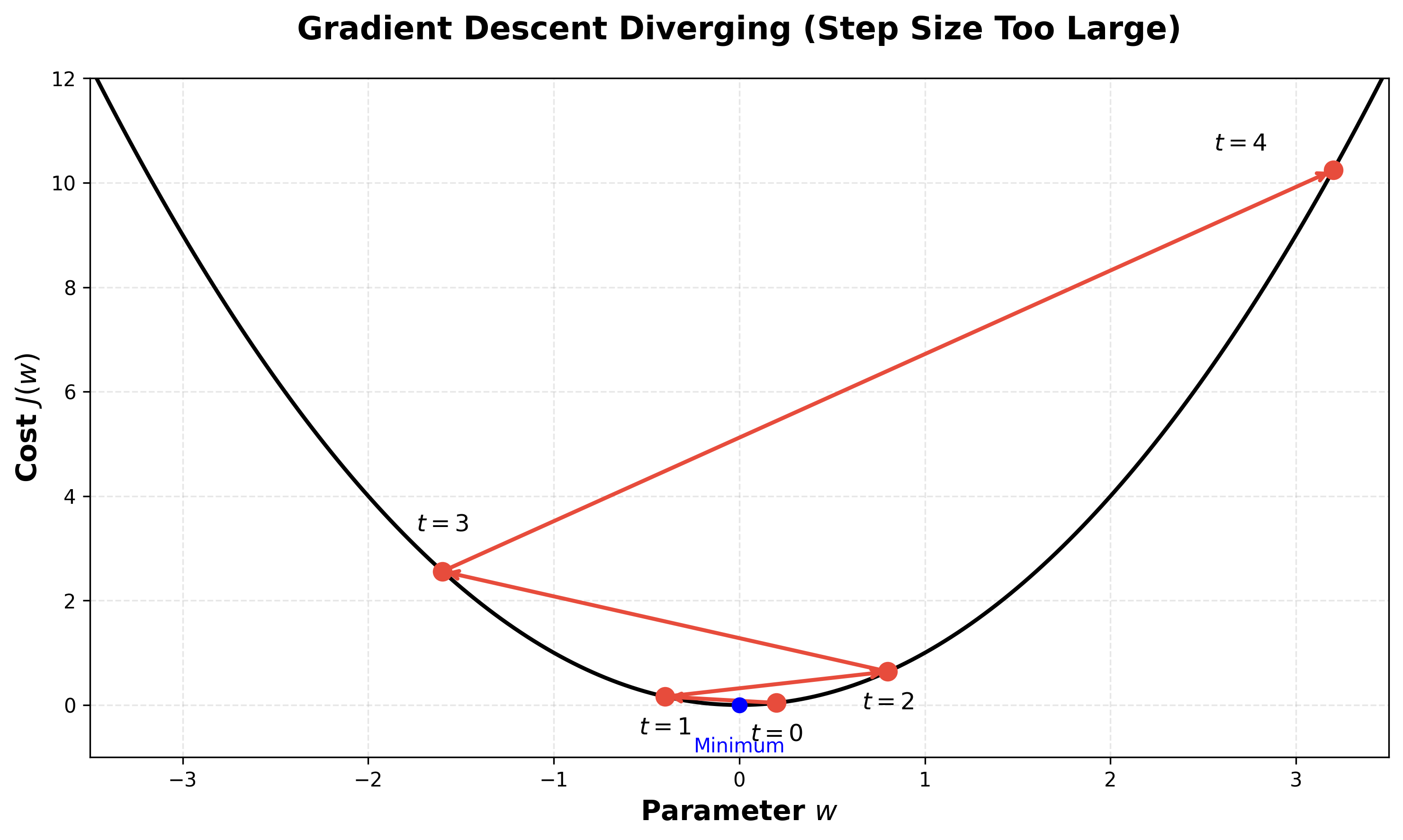
Learning Rate
The size of the steps taken during gradient descent is called the learning rate. It's a critical hyperparameter:
- A high learning rate can cover more ground but risks overshooting the minimum.
- A low learning rate is more precise but can take a very long time to converge.
Model Validation: Cross-Validation
To get a more reliable estimate of our model's performance on unseen data, we use k-fold cross-validation. The process is:
- Split the training data into 'k' equal-sized folds (e.g., k=5).
- Train the model 'k' times. In each iteration, use one fold as the validation set and the remaining k-1 folds as the training set.
- The final performance metric is the average of the metrics from the 'k' folds.
This gives a more robust estimate of how the model will perform and helps prevent overfitting.