Feature Selection and Engineering
In machine learning, not all columns in your dataset are equally useful. The goal of this stage is to select the most impactful input variables (Feature Selection) and create new, more informative ones from the existing data (Feature Engineering). Getting this right is critical for building an accurate and efficient model.
Benefits of good feature selection and engineering include:
- Reduces Overfitting: Less redundant data means less opportunity for the model to learn from noise.
- Improves Accuracy: A model with the right features can better capture the true signal in the data.
- Reduces Training Time: Fewer features mean the model trains faster.
Feature Selection Techniques
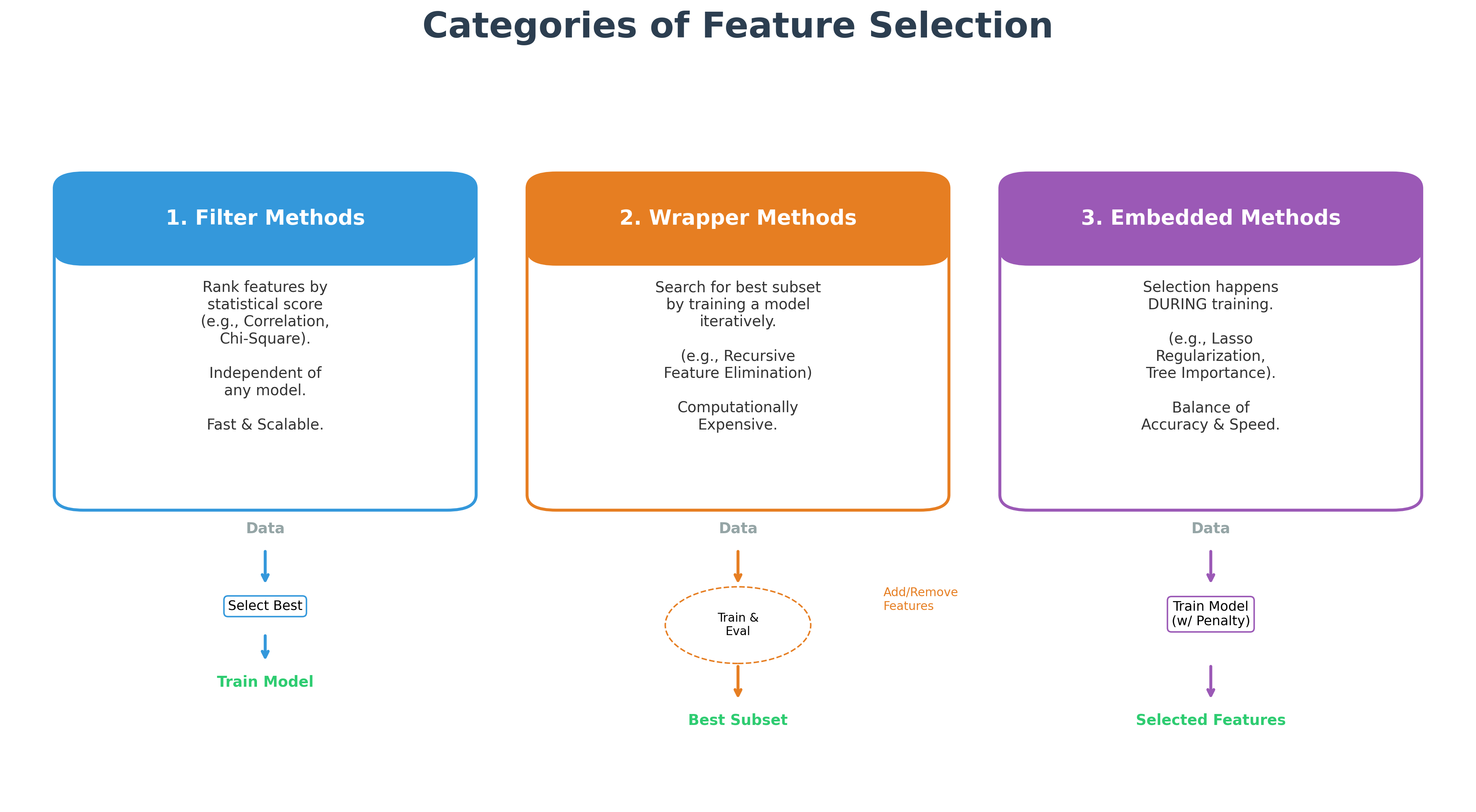
Feature selection methods can be grouped into three main categories:
1. Filter Methods
These techniques analyze the statistical properties of each feature and rank them before any model is built. They are fast and computationally inexpensive.
- Correlation: You can calculate the correlation (e.g., Pearson correlation) between each independent variable and the target variable. Features with very low correlation can often be dropped.
- SelectKBest: Scikit-learn's
SelectKBestis a versatile tool that can use various statistical tests to select a specific number ('k') of the most powerful features.
2. Wrapper Methods
These methods use a specific machine learning model to evaluate the usefulness of a subset of features. They are more computationally expensive but can lead to better model performance.
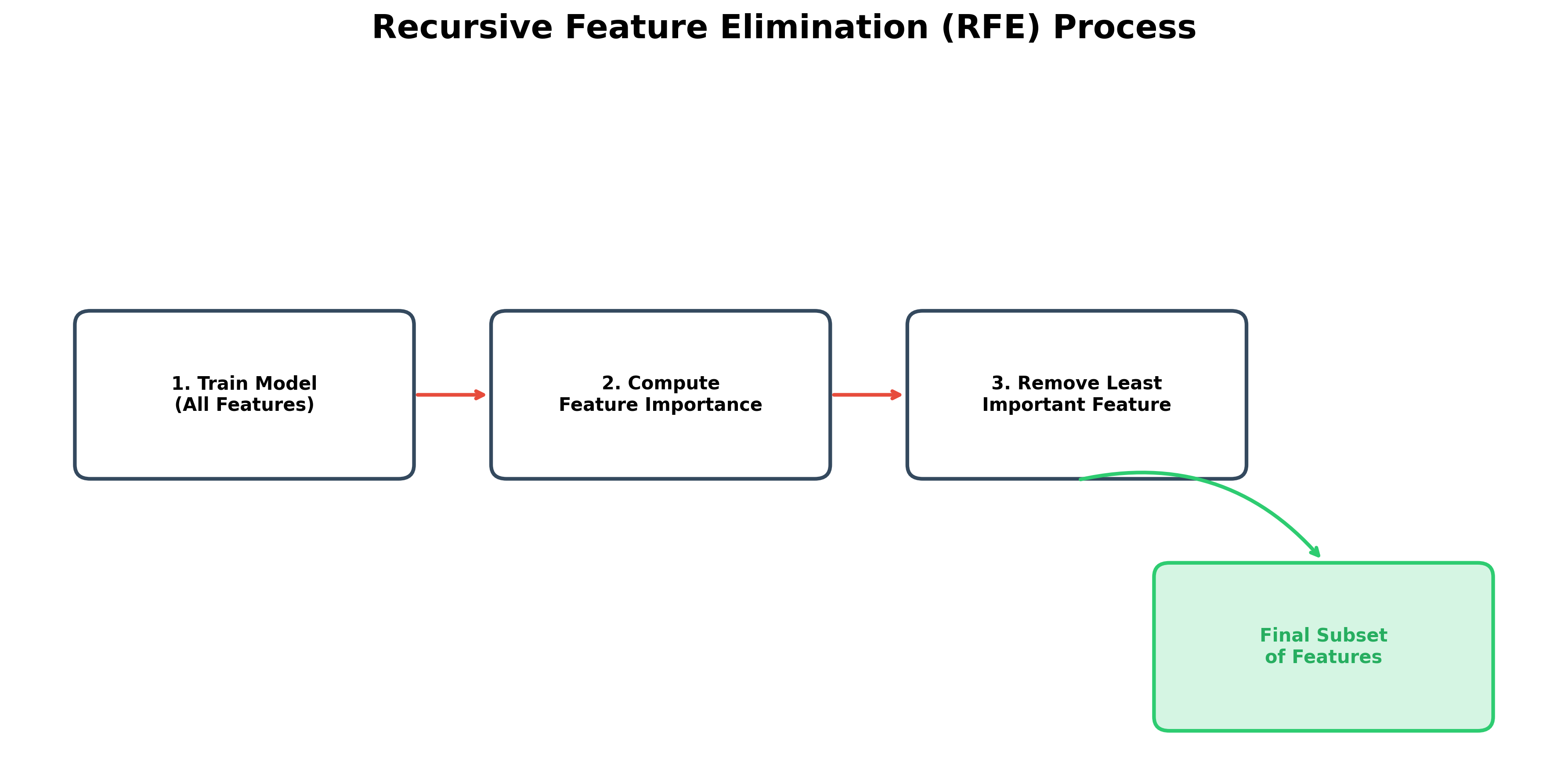
Recursive Feature Elimination (RFE): This method starts with all features, builds a model, and removes the weakest feature. It repeats this process until the desired number of features is left.
Forward Selection: This is the opposite of RFE. It starts with no features and iteratively adds the feature that most improves the model's performance until no significant improvement is gained.
3. Embedded Methods
These methods perform feature selection as part of the model training process itself.
- L1 (Lasso) Regularization: As mentioned in the 'Model Building' chapter, Lasso regularization can shrink the coefficients of less important features to zero, effectively removing them from the model.
- Tree-Based Importance: Models like Random Forest and Gradient Boosting naturally calculate an 'importance' score for each feature based on how much it contributes to the model's accuracy. You can use these scores to rank and select the most influential features.
Handling Multicollinearity
Multicollinearity occurs when two or more independent variables are highly correlated with each other. This can make it difficult for a model to determine the individual effect of each variable.
To identify these relationships, you can use the Variance Inflation Factor (VIF). VIF measures how much a feature is inflated by its correlation with other features. A high VIF score for a variable indicates that it is highly collinear and could be a candidate for removal.
While multicollinearity does not always reduce a model's overall predictive power, it can make the model's coefficients unstable and difficult to interpret.
Dimensionality Reduction using Principal Component Analysis (PCA)
Principal Component Analysis (PCA) is a dimensionality reduction technique. Unlike feature selection, which picks a subset of existing columns, PCA creates entirely new, artificial features called Principal Components (PC).
How PCA Works (The "Distillation" Process)
Imagine you have a dataset with several columns. Let's look at a small sample of the raw data:
| Measurement | Subject A | Subject B | Subject C | Subject D | Subject E |
|---|---|---|---|---|---|
| Height (m) | 1.73 | 1.84 | 1.54 | 1.68 | 1.88 |
| Weight (kg) | 78 | 65 | 69 | 75 | 90 |
| Blood Pressure | 120 | 110 | 90 | 130 | 150 |
Many of these columns are highly correlated—they essentially tell the same story.
- Finding Correlations: PCA looks for these overlapping stories. In the table above, notice that as Height and Weight increase (Subject E), Blood Pressure often follows.
- Merging Information: It "squashes" the correlated features together into new, artificial axes called Principal Components.
- Capturing Variance:
- PC1 (The Grand Summary): This axis captures the most important trend in the data. For example, if "Overall Size" accounts for the biggest difference between your subjects, PC1 will represent size.
- PC2 (The Secondary Detail): this axis captures the next most important trend that PC1 missed (e.g., "Health Indicators" like Blood Pressure).
Understanding the Axes: PC1 vs. PC2
When PCA creates these new axes, it follows a strict hierarchy:
- PC1 (Principal Component 1): This is the "Grand Summary" axis. It is mathematically calculated to capture the maximum amount of variance (spread) in your data. If your data was a cloud of points, PC1 would be the longest line you could draw through the middle of that cloud.
- PC2 (Principal Component 2): This is the "Secondary Detail" axis. It is drawn at a 90-degree angle to PC1 and captures the next most important pattern that PC1 missed.
Why do we only use 2 axes?
Technically, PCA creates a new axis for every column in your original data. If you had 50 columns, you would have PC1 through PC50. However, we usually discard most of them and keep only the first two or three because:
- Information Density: PC1 and PC2 usually capture the "meat" of the data (often 80-90% of the total variance).
- Visualization: We use 2 axes because it allows us to project a complex, high-dimensional problem onto a simple 2D map that humans can actually see and understand.
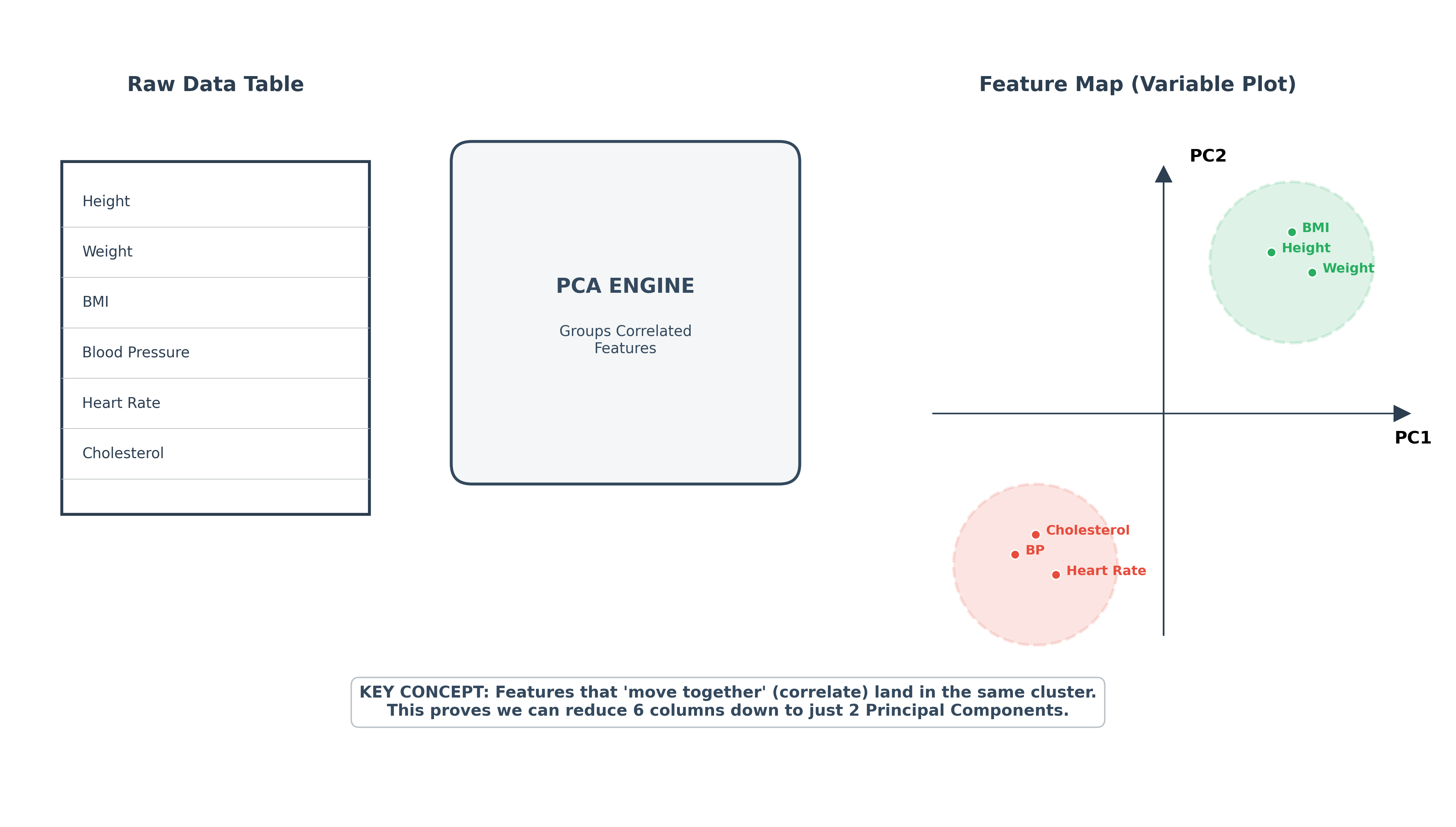
Why do Clusters Appear? (Feature Mapping)
In the diagram below, notice that the dots are the features themselves (like Height, Weight, Blood Pressure).
- The Concept: When features are highly correlated, they are mathematical "twins." Because they move together in the raw data, PCA places them very close to each other on the map.
- The Green Cluster: Height, Weight, and BMI all cluster together because they collectively describe "Body Size."
- The Red Cluster: Blood Pressure, Heart Rate, and Cholesterol cluster together because they describe "Cardiovascular Health."
- Dimensionality Reduction: Because these features cluster so tightly, we can stop using all 6 individual columns and instead use just 2 Principal Components (PC1 and PC2) to represent the entire "Body Size" and "Health" stories.
PCA is an unsupervised technique that is incredibly powerful for simplifying complex datasets before feeding them into a machine learning model.
Feature Engineering
Feature engineering is the creative process of using domain knowledge to create new features from your existing data. The goal is to generate variables that better represent the underlying problem and improve model performance. Examples include:
- Combining & Aggregating Features:
- Creating a 'total rooms' feature by adding 'bedrooms' and 'bathrooms'.
- Summing
toll_amountandfare_amountto calculate atotal_fare. - Calculating dollars spent over a week, month, or year in time-series data to capture trends and seasonality (e.g., holiday sales).
- Calculating Differences (Time & Physical):
- Employee Churn: Instead of using two raw dates (today and date of last raise), engineer a single feature representing the "time elapsed since last raise."
- Vehicle Diagnostics: Finding the difference between tire pressures to derive weight distribution or analyze gradients on different surfaces.
- Decomposing & Extracting:
- Splitting a 'datetime' column into 'year', 'month', 'day', and 'day_of_week' (e.g., taxi fares often vary significantly by weekday).
- Extracting the first letter of a domain from a full URL to reduce complexity.
- Handling High Cardinality:
- Grouping: Instead of tracking thousands of individual referral websites, group them into categories like "News," "Social Media," etc.
- Hashing: Using feature hashing to convert high-cardinality features into a fixed-size vector.
- Binning & Bucketizing:
- Converting continuous numerical features like 'age' into categorical bins ('child', 'adult', 'senior').
- Geospatial Bucketing: Dividing latitude and longitude into grid squares to create categorical location features.
- Outlier Filtering as Engineering: Improving model focus by removing records that fall outside domain-specific boundaries, such as:
- Filtering taxi trips to stay within city limits (e.g., NYC boundaries).
- Removing illogical records like fares under $2 or trips with zero passengers.
- Encoding: As discussed previously, encoding categorical variables is also a form of feature engineering.
- Concatenating multiple feature transformations using scikit-learn's
FeatureUnion.
Feature selection and engineering are often more of an art than an exact science, and honing these skills comes with practice. Many ML solutions fail not because of the model chosen, but because of poor feature selection and engineering.
Note: Based on the use case, an independent variable or feature may be called a predictor variable, regressor, explanatory variable, etc. The dependent variable is also known as a response variable, outcome variable, target, or label.
Reference: https://medium.com/analytics-vidhya/feature-selection-techniques-2614b3b7efcd https://www.analyticsvidhya.com/blog/2020/10/feature-selection-techniques-in-machine-learning/