Training Neural Networks
Training a neural network is an optimization problem. The goal is to find the set of weights and biases that minimizes a loss function, which measures how far the model's predictions are from the actual truth. The primary algorithm used to achieve this is Gradient Descent.
Loss Functions: Measuring the Error
As discussed in Loss Functions & Optimization, there is a technical distinction between a loss function (error for one sample) and a cost function (average error over the dataset).
In practice, the term "loss" is often used to refer to both, including in PyTorch code. For example, a "loss function" in code typically returns the mean error for a mini-batch (which is technically a cost).
def loss(y_predicted, y_actual):
  # Technically calculates the Mean Squared Error (Cost) for a batch
  return ((y_predicted - y_actual)**2).mean()
Gradient Descent: Finding the Minimum
Gradient Descent is the iterative optimization algorithm used to find the minimum of the cost function.
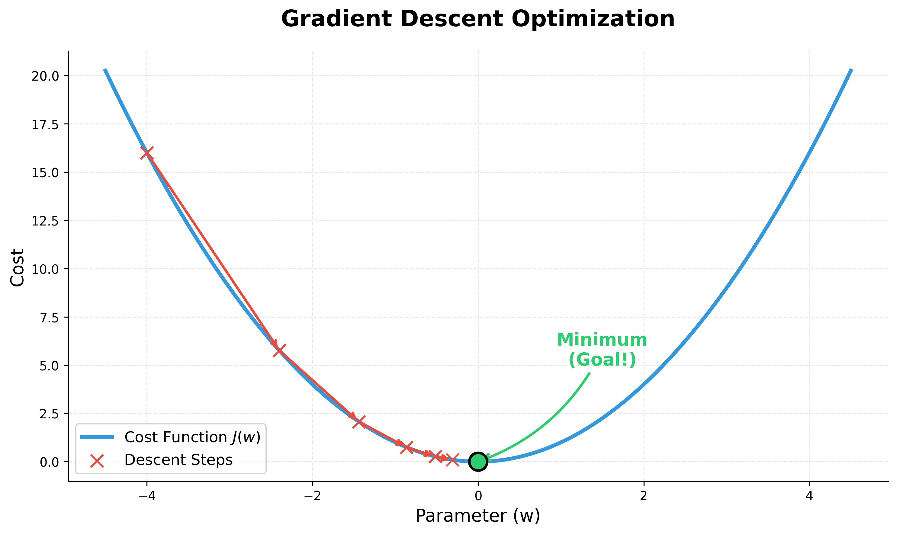
While the basic intuition is like walking down a hill, the training process for a neural network involves these specific steps:
- Start with random values for the model's parameters (weights and biases).
- Calculate the gradient of the cost function with respect to each parameter.
- Update each parameter by taking a small step in the opposite direction of the gradient, controlled by a learning rate.
- Repeat until the cost stops decreasing significantly.
Stochastic Gradient Descent (SGD)
In practice, calculating the gradient using the entire dataset can be very slow. Stochastic Gradient Descent (SGD) is a variation where the gradient is calculated on a small, random subset of the data called a mini-batch.
This makes the process much faster and can also help the model escape shallow local minima.
Optimizers in PyTorch
PyTorch's torch.optim package provides a wide variety of optimization algorithms, including SGD. An optimizer takes the model's parameters and a learning rate as input and handles the process of updating the parameters based on the computed gradients.
Here's how to use an SGD optimizer in PyTorch:
import torch

# Assume 'model' is an nn.Module with parameters
# lr is the learning rate
optimizer = torch.optim.SGD(model.parameters(), lr=0.01)

# Inside the training loop...
for inputs, labels in dataloader:
    # 1. Clear old gradients
    optimizer.zero_grad()

    # 2. Forward pass: compute predicted outputs
    outputs = model(inputs)

    # 3. Calculate the loss
    loss = criterion(outputs, labels) # criterion is the loss function

    # 4. Backward pass: compute gradients
    loss.backward()

    # 5. Update the weights
    optimizer.step()
The training loop consists of these five core steps, repeated for a number of epochs (passes over the entire dataset).
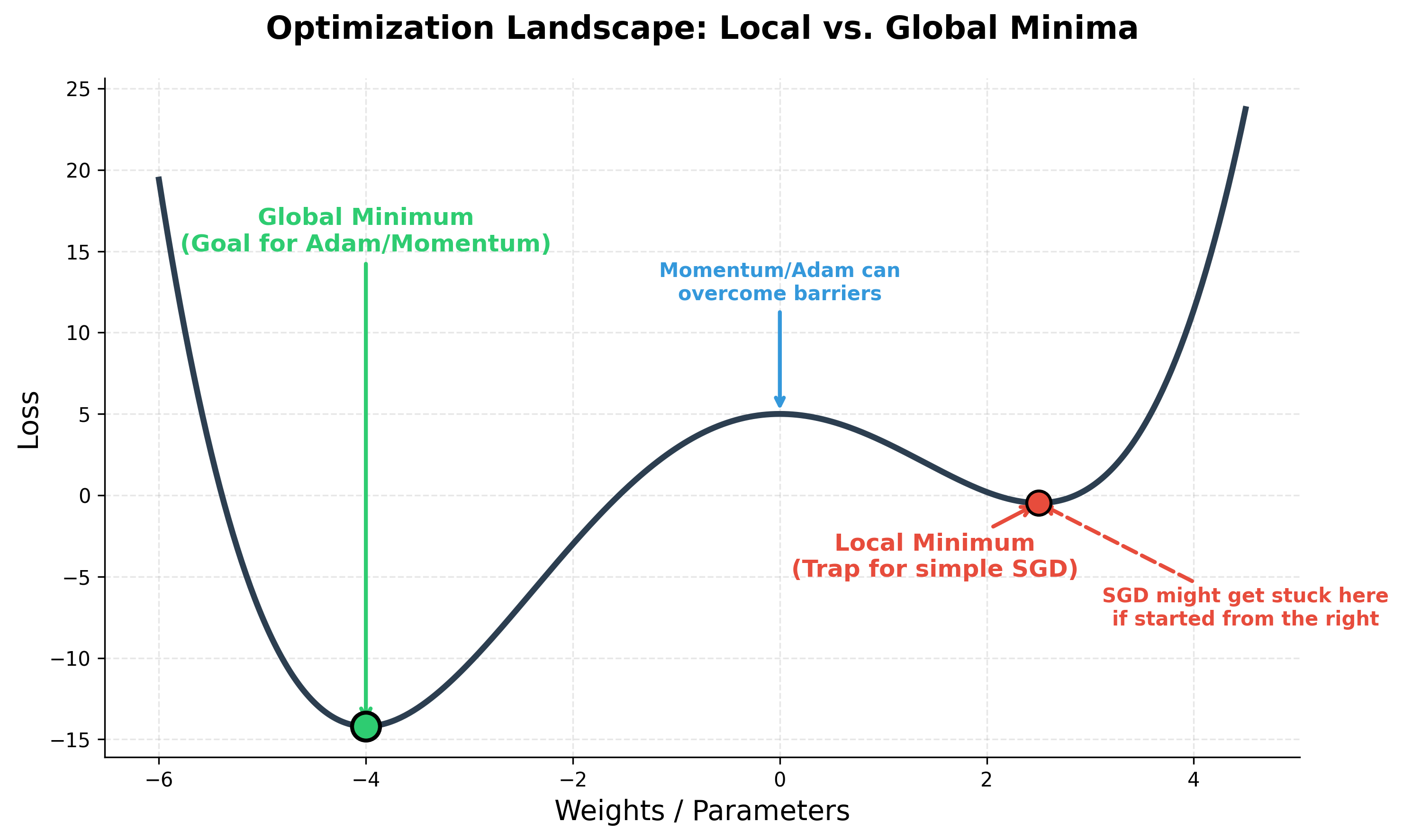
Beyond SGD: Adaptive Optimizers
While SGD is powerful, it has limitations. One major challenge in training deep neural networks is the complex landscape of the loss function. It often contains many local minima—valleys that look like the bottom but aren't the lowest point (the global minimum).
Standard SGD can easily get stuck in these local minima or saddle points (flat areas). It also struggles when the loss changes quickly in one direction and slowly in another (a ravine).
To overcome these issues, researchers have developed more advanced optimizers:
1. Momentum
Momentum helps SGD accelerate in the relevant direction and dampens oscillations. It does this by adding a fraction of the update vector of the past time step to the current update vector. Think of a heavy ball rolling down a hill; it gathers momentum and doesn't get stuck in small bumps.
2. RMSProp
RMSProp (Root Mean Square Propagation) adapts the learning rate for each parameter. It divides the learning rate by an exponentially decaying average of squared gradients. This means parameters with large gradients have their learning rate reduced, and those with small gradients have it increased, balancing the step sizes.
3. Adam (Adaptive Moment Estimation)
Adam is currently one of the most popular optimizers. It combines the best ideas of Momentum and RMSProp:
- It keeps track of an exponentially decaying average of past gradients (like Momentum).
- It keeps track of an exponentially decaying average of past squared gradients (like RMSProp).
This makes Adam very fast and effective for a wide range of problems, often converging to a good solution (near the global minimum) much faster than plain SGD.
# Using Adam in PyTorch is just as easy as SGD
optimizer = torch.optim.Adam(model.parameters(), lr=0.001)
Pro Tip: When to use which? If Adam is so much faster and better at navigating local minima, why would we ever use simple SGD?
- Generalization: While Adam is faster, research suggests that SGD with Momentum often finds "flatter" minima that generalize better to new, unseen data. In many state-of-the-art computer vision models (like ResNet), SGD is still the gold standard for achieving the highest final accuracy.
- Memory Efficiency: Adam stores two additional variables for every parameter in your model, which increases memory usage. SGD is much more lightweight.
- The Verdict: Start with Adam for quick results and experimentation. If you are pushing for a world-class, high-accuracy model and have the time to tune the learning rate carefully, consider switching to SGD + Momentum for the final polish.
Datasets and DataLoaders
Data is the fuel for neural networks. To make managing and iterating over this fuel efficient, PyTorch provides two primitive classes: Dataset and DataLoader.
1. Dataset
The Dataset class stores the samples and their corresponding labels. You can use pre-built datasets (like TensorDataset) or create your own custom class to load images or text files from disk on demand.
2. DataLoader
The DataLoader wraps an iterable around the Dataset. It is the engine that feeds data to your model.
Why is DataLoader so important?
You could write a for loop to iterate over your data manually, but DataLoader automates several critical optimizations:
- Batching: Instead of feeding one sample at a time, it groups data into "mini-batches" (e.g., 32 or 64 samples). GPUs are massive parallel processors; feeding them batches allows them to process multiple samples simultaneously, drastically speeding up training.
- Shuffling: It automatically shuffles the data at the start of every epoch. This is vital to ensure the model doesn't learn order-dependent patterns (e.g., remembering that "all cats are in the first half of the dataset").
- Parallel Multiprocessing: Loading and processing large images can be slow.
DataLoadercan use multiple CPU cores (num_workers) to pre-load data in the background while the GPU is busy training on the current batch. This pipeline ensures the GPU never sits idle waiting for data.
from torch.utils.data import TensorDataset, DataLoader
import torch

# Create a dataset from tensors
x_train = torch.randn(100, 10)
y_train = torch.randn(100, 1)
train_ds = TensorDataset(x_train, y_train)

# Create a data loader to iterate over the dataset in batches
# shuffle=True ensures data is mixed every epoch
# batch_size=128 processes 128 samples at once
train_dl = DataLoader(train_ds, batch_size=128, shuffle=True)

# Now you can loop over the data loader in your training loop
for x_batch, y_batch in train_dl:
    pass  # ... training steps ...