Multilayer Perceptrons (MLPs)

A Multilayer Perceptron (MLP) is the classic type of feedforward artificial neural network. It consists of an input layer, an output layer, and one or more hidden layers in between. These hidden layers are what give the MLP its ability to learn complex, non-linear patterns.

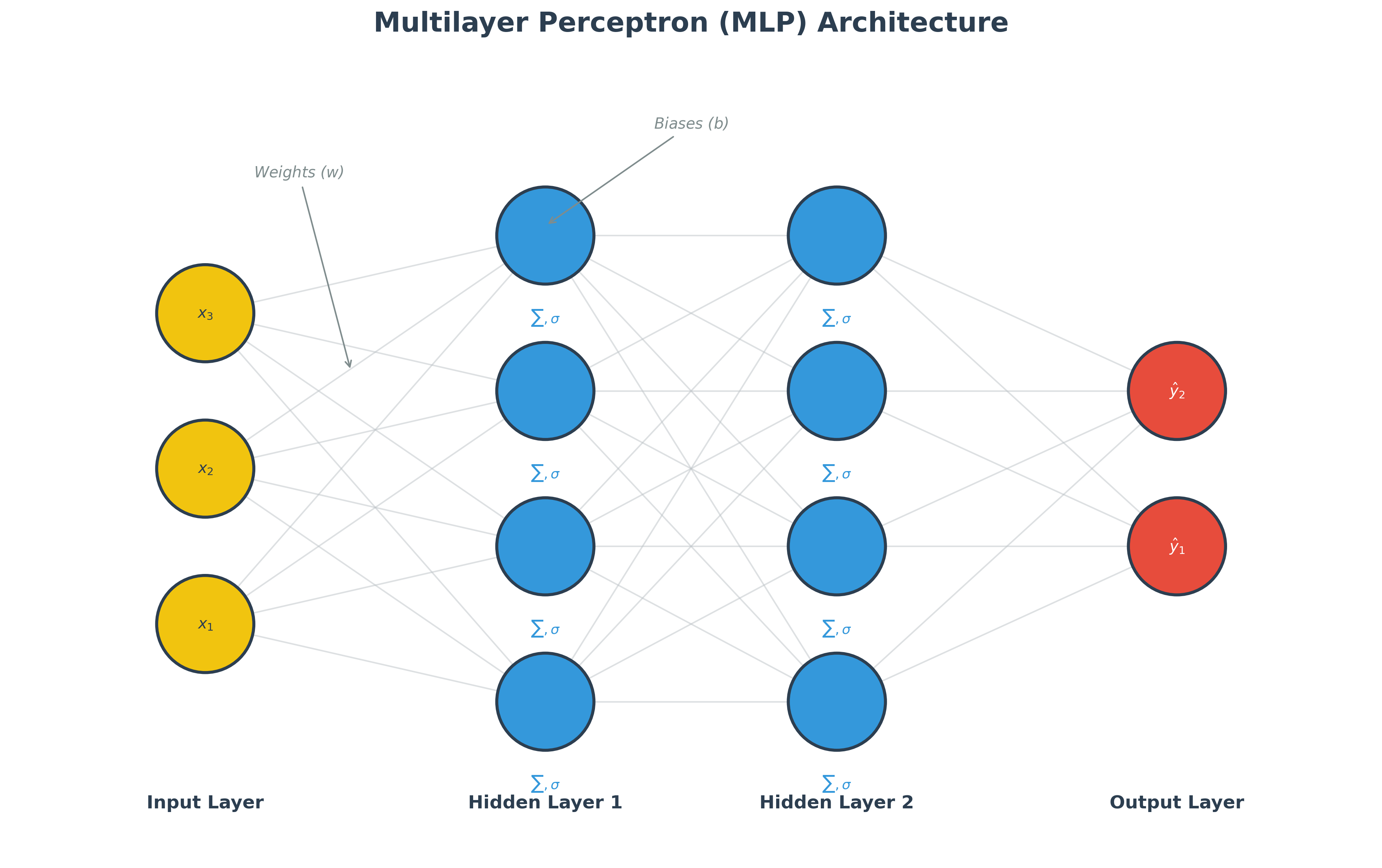
The Components of an MLP

As shown in the diagram above, an MLP consists of several key elements:

• Input Layer ($x$): Receives the raw data. Each node represents a single feature from your dataset.
• Weights ($w$): These are the connections between neurons. They determine the "importance" of a piece of information as it travels through the network.
• Hidden Layer ($\sum, \sigma$): This is where the learning happens. Each neuron calculates a weighted sum of its inputs and then applies a non-linear activation function ($\sigma$) to decide what information to pass forward.
• Biases ($b$): An additional value added to the weighted sum, acting like an "offset" to help the model better fit the data.
• Output Layer ($\hat{y}$): The final stage that produces the prediction (e.g., a classification label or a numeric value).

From Linear to Non-Linear

A simple model with only an input and output layer can only learn linear relationships. For example, it could fit a line to data, but it could not model a curve.

To capture non-linear patterns, we introduce hidden layers and activation functions.

Activation Functions: Introducing Non-Linearity

An activation function is a function applied to the output of each neuron. Its purpose is to introduce non-linearity into the network. Without a non-linear activation function, a deep neural network would behave just like a single-layer linear model, no matter how many layers it has.

There are many types of activation functions, but some of the most common are:

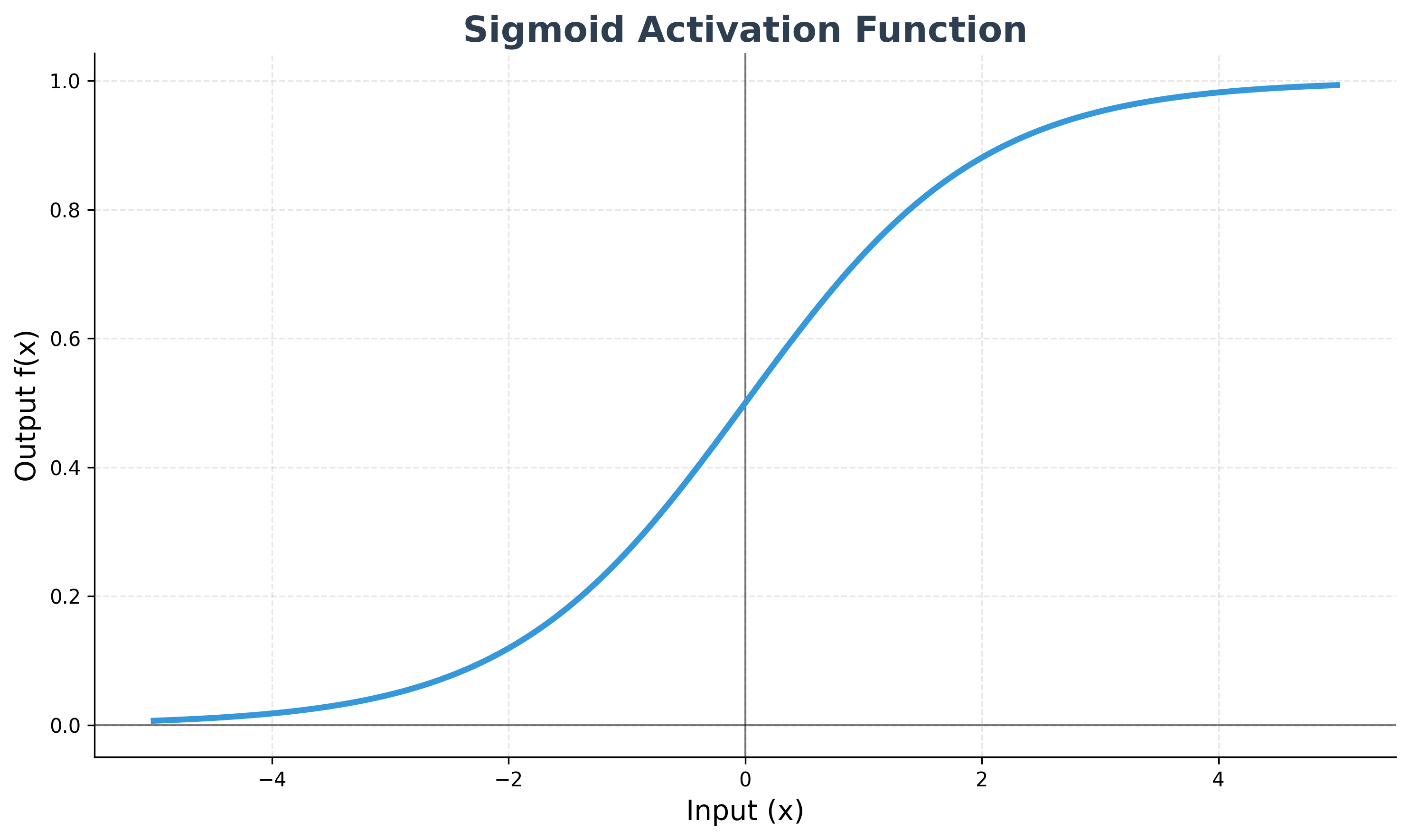
Sigmoid

The sigmoid function squashes its input into a range between 0 and 1. It was historically popular but is less used in hidden layers today due to the vanishing gradient problem.

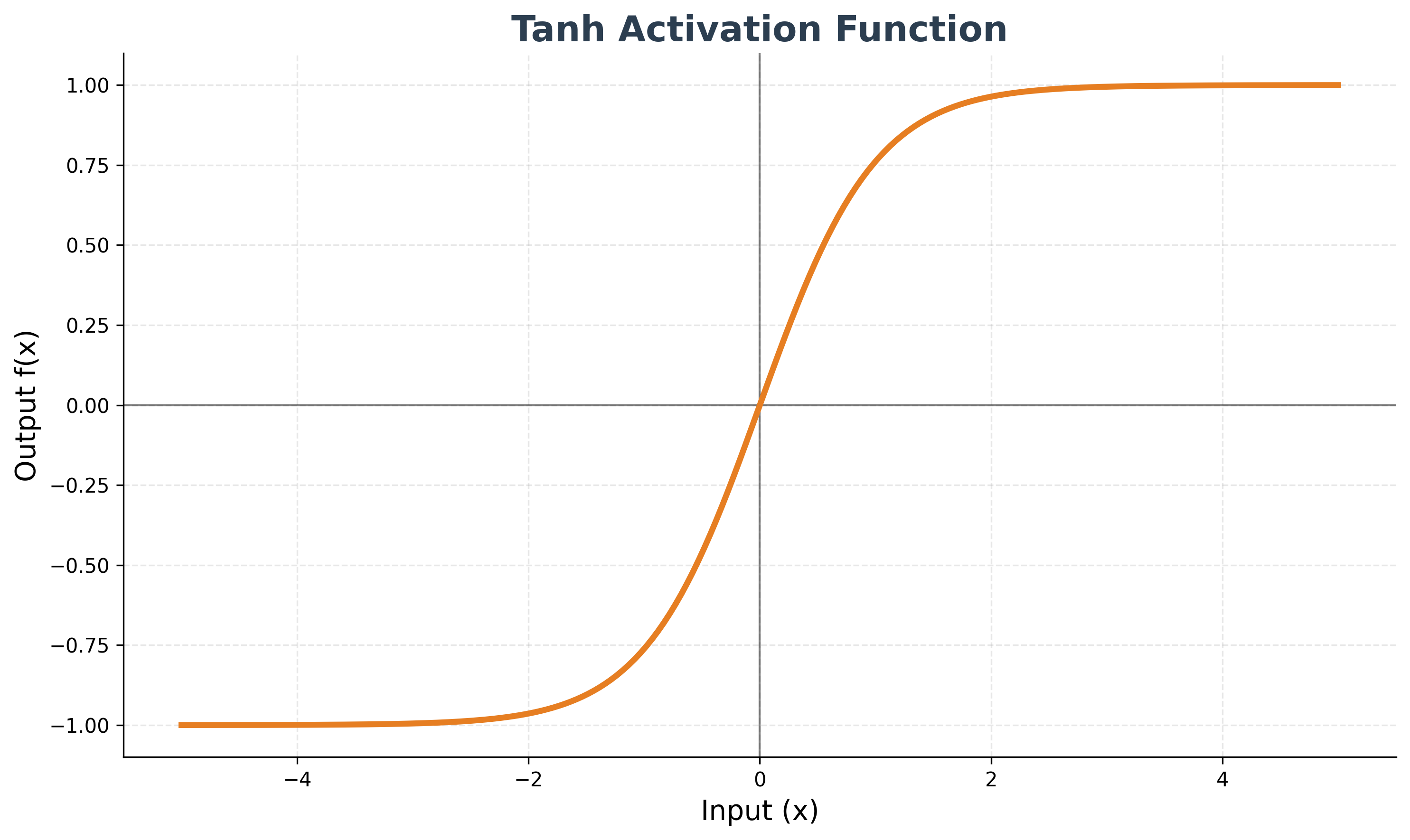
Tanh (Hyperbolic Tangent)

Tanh is similar to sigmoid but squashes its input into a range between -1 and 1. It is also susceptible to the vanishing gradient problem.

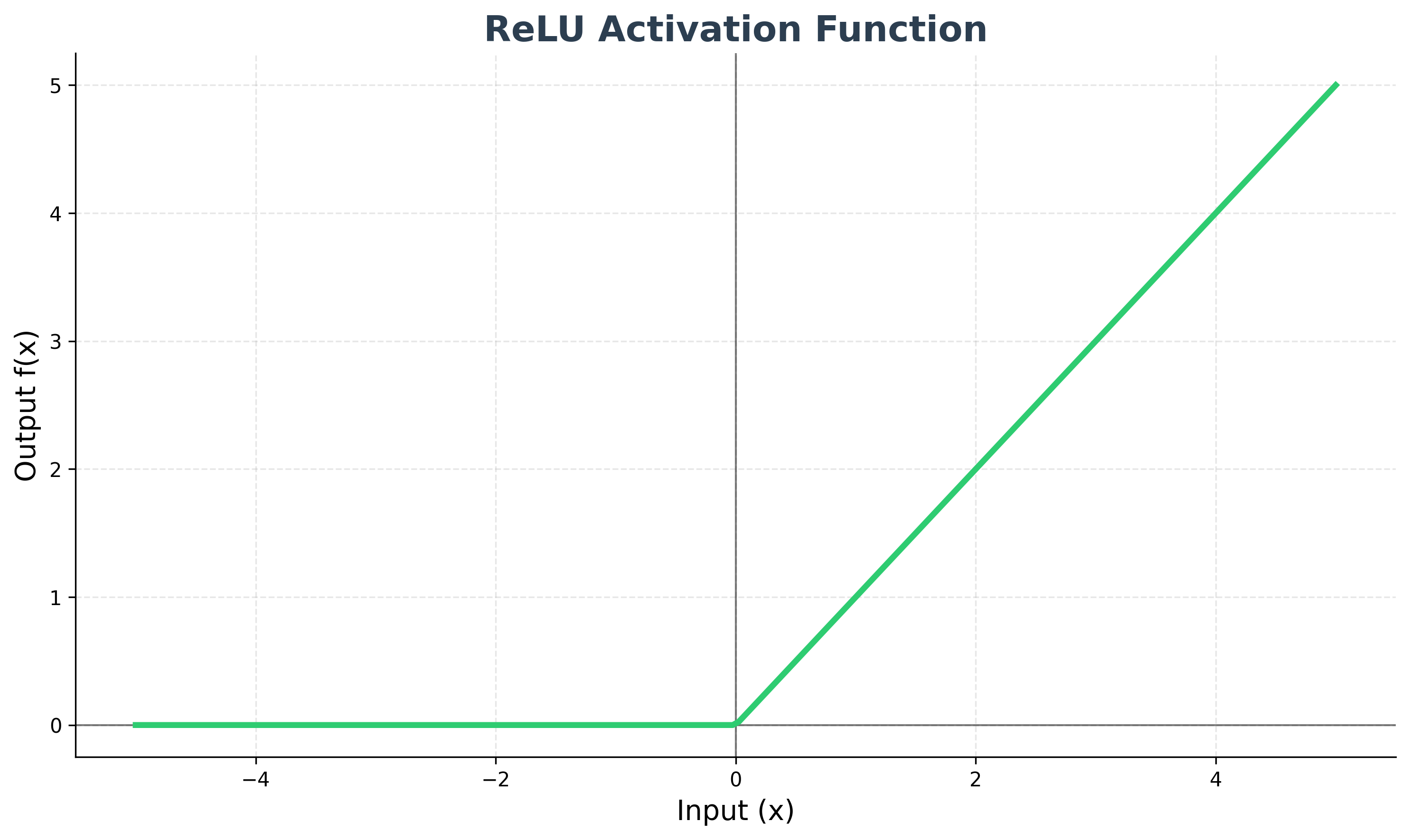
ReLU (Rectified Linear Unit)

ReLU is the most popular activation function for hidden layers in modern neural networks. It is defined as f(x) = max(0, x). It is computationally very efficient and helps to alleviate the vanishing gradient problem.

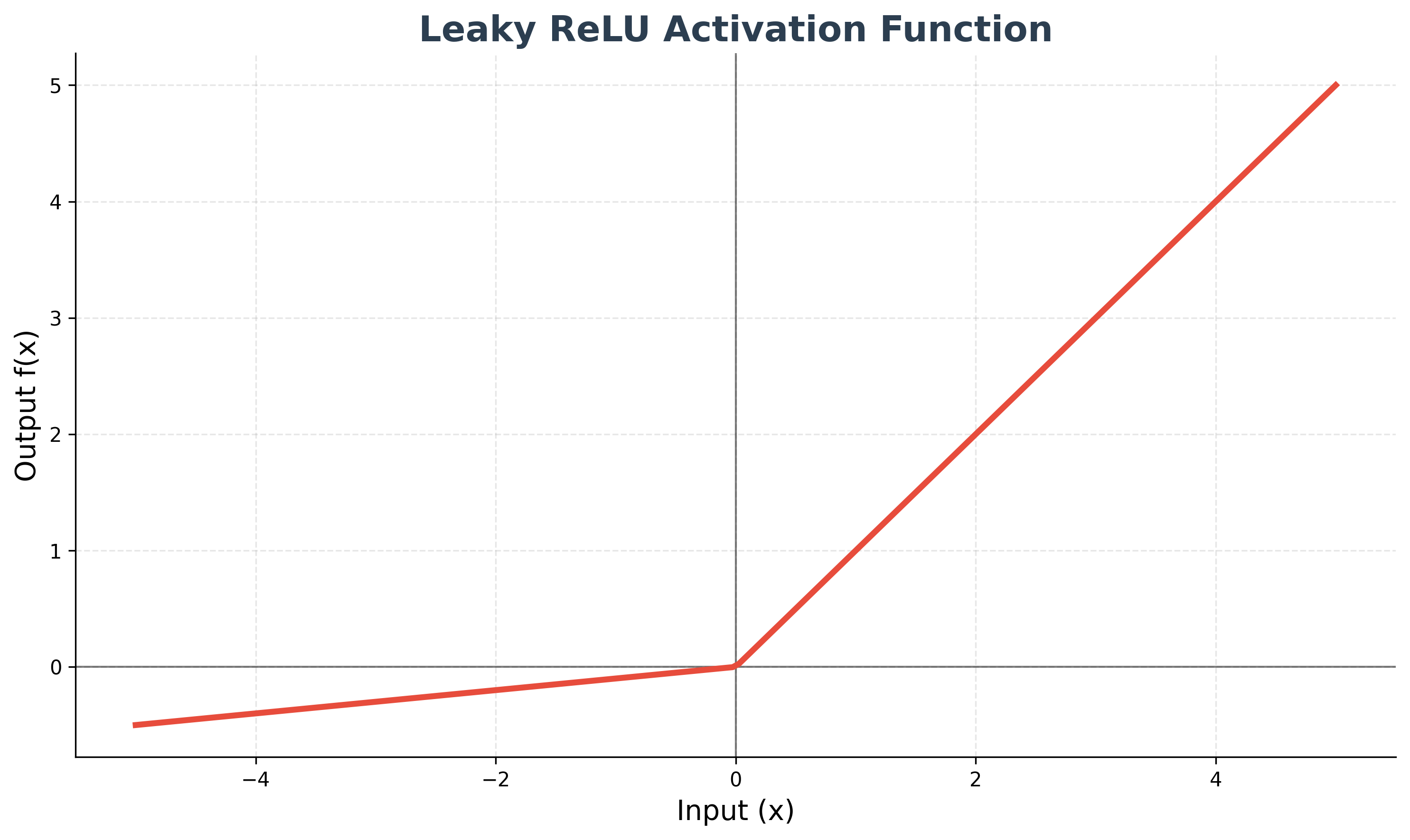
Leaky ReLU

Leaky ReLU is a variation of ReLU that allows a small, non-zero gradient when the input is negative (f(x) = x if x > 0, else 0.01x). This helps to prevent "dying ReLU" neurons, which can happen if a neuron gets stuck in the negative region and stops learning.

Building an MLP in PyTorch

PyTorch's nn.Module makes it easy to build an MLP. We define the layers in the __init__ method and specify how data flows through them in the forward method.

Here is an example of a simple MLP with one hidden layer:

import torch
from torch import nn
import torch.nn.functional as F

class SimpleMLP(nn.Module):
    def __init__(self, input_size, hidden_size, output_size):
        super().__init__()
        # Define the layers
        self.hidden_layer = nn.Linear(input_size, hidden_size)
        self.output_layer = nn.Linear(hidden_size, output_size)

    def forward(self, x):
        # Define the forward pass
        x = self.hidden_layer(x)
        # Apply the ReLU activation function
        x = F.relu(x)
        x = self.output_layer(x)
        return x

Using nn.Sequential for Simpler Models

For simple, feedforward networks, you can use nn.Sequential to create a model more compactly.

hidden_dim = 32
model = nn.Sequential(
    nn.Linear(p, hidden_dim),
    nn.ReLU(),
    nn.Linear(hidden_dim, 1)
)

This creates the same network as the class-based example above, but with less code. The class-based approach is more flexible for complex architectures where data might not flow in a simple straight line.

Softmax: For Multi-Class Classification

When you have a classification problem with more than two classes (e.g., classifying handwritten digits 0-9), you need a way to output a probability distribution across all the classes. The Softmax function is used for this.

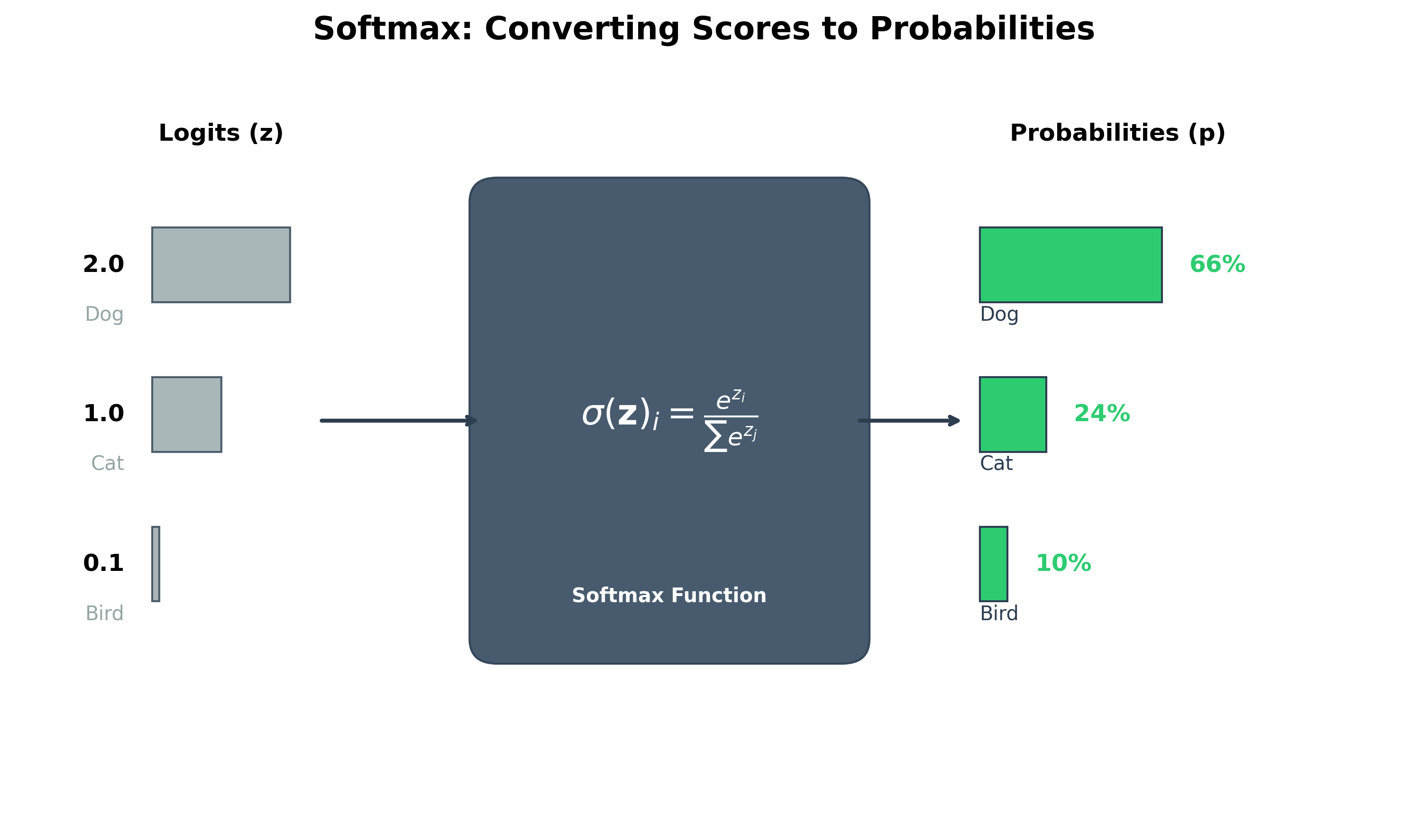
It takes a vector of raw scores (called logits) from the final layer of the network and converts them into a vector of probabilities that sum to 1.

The class with the highest probability is the model's prediction. The loss function typically used with Softmax is Cross-Entropy Loss, which measures the difference between the predicted probability distribution and the true distribution.