Regularization: Preventing Overfitting
One of the most common challenges in training deep neural networks is overfitting. This occurs when a model learns the training data too well, capturing not only the underlying patterns but also the noise and random fluctuations. An overfit model performs very well on the data it was trained on, but fails to generalize to new, unseen data.
Demonstrating Overfitting
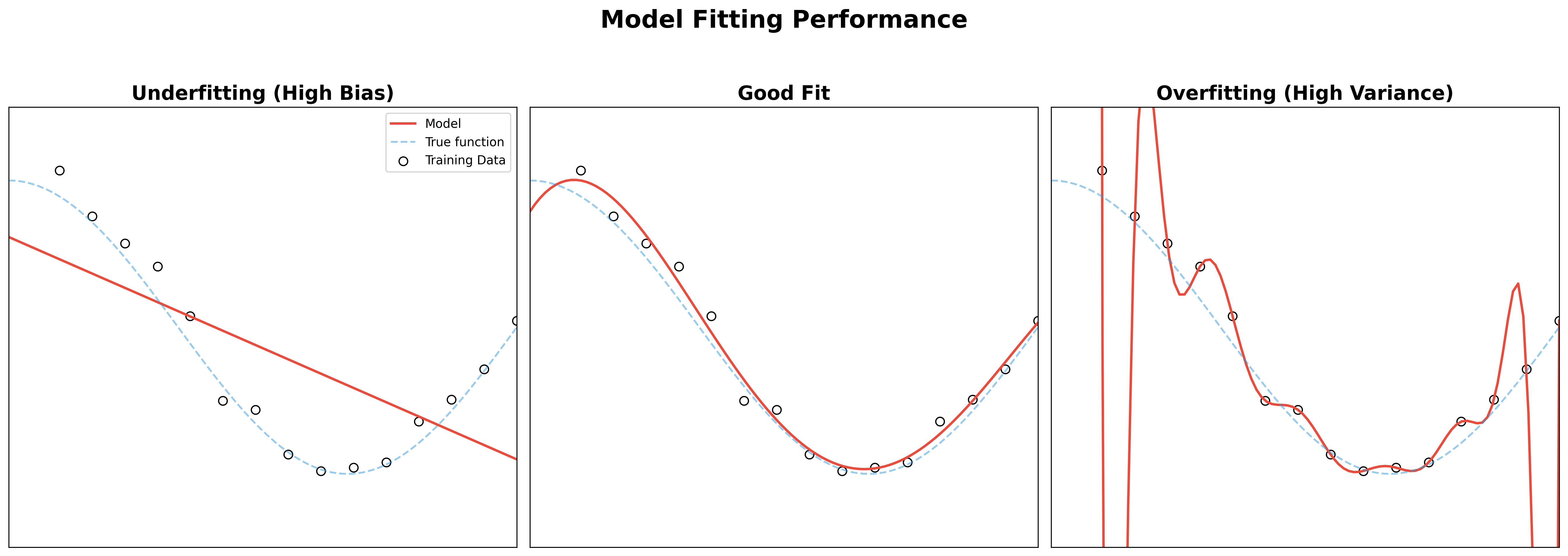
To truly understand regularization, we must first see how overfitting manifests during training. Overfitting occurs when a model learns the specific noise and fluctuations in the training data to the extent that it negatively impacts its performance on new data.
1. Training vs. Validation Metrics
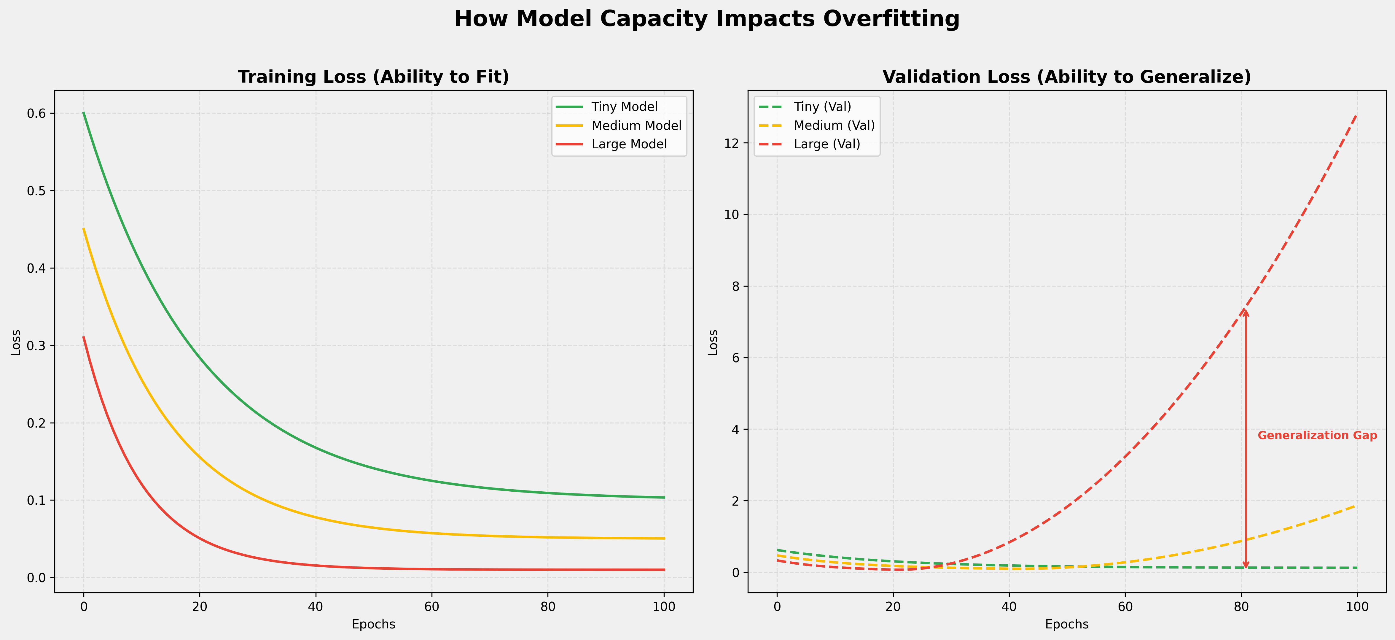
When a model begins to overfit, you will notice a divergence in its performance metrics:
- Training Loss: Continues to decrease as the model gets better at "memorizing" the training set.
- Validation Loss: Stops decreasing and starts to increase. This indicates that while the model is becoming a "perfect dictionary" for the training data, it is losing its ability to generalize to unseen examples.
The difference between the training and validation performance is known as the Generalization Gap.
2. The Impact of Model Capacity
A model's "capacity" refers to the number of learnable parameters it has. The relationship between capacity and overfitting is a critical intuition:
- Smaller Models (Low Capacity): Have fewer parameters and are forced to learn compressed, more meaningful representations of the data. They are naturally more robust to overfitting because they don't have enough "memory" to store the noise.
- Larger Models (High Capacity): Have ample parameters to memorize the entire training set, including random noise. They overfit much more quickly and severely.
As discussed in Model Building Concepts, regularization refers to a set of techniques designed to prevent this behavior and improve a model's ability to generalize.
The goal is to find a "sweet spot" where the model is complex enough to capture the true patterns in the data, but not so complex that it learns the noise.
L1 Regularization (Lasso)
L1 Regularization (Least Absolute Shrinkage and Selection Operator) adds a penalty term to the loss function that is proportional to the absolute value of the magnitude of the weights.
Key characteristics of L1:
- Feature Selection: It has the effect of pushing the weights of less important features exactly to zero. This effectively performs feature selection, resulting in a sparse model.
- Robustness: It is generally more robust to outliers than L2 regularization.
L2 Regularization (Ridge / Weight Decay)
L2 Regularization adds a penalty term to the loss function that is proportional to the square of the magnitude of the weights. This is based on the principle of Structural Risk Minimization, where we aim to minimize:
The L2 complexity is defined as the sum of squared weights:
The Role of Lambda (\lambda)
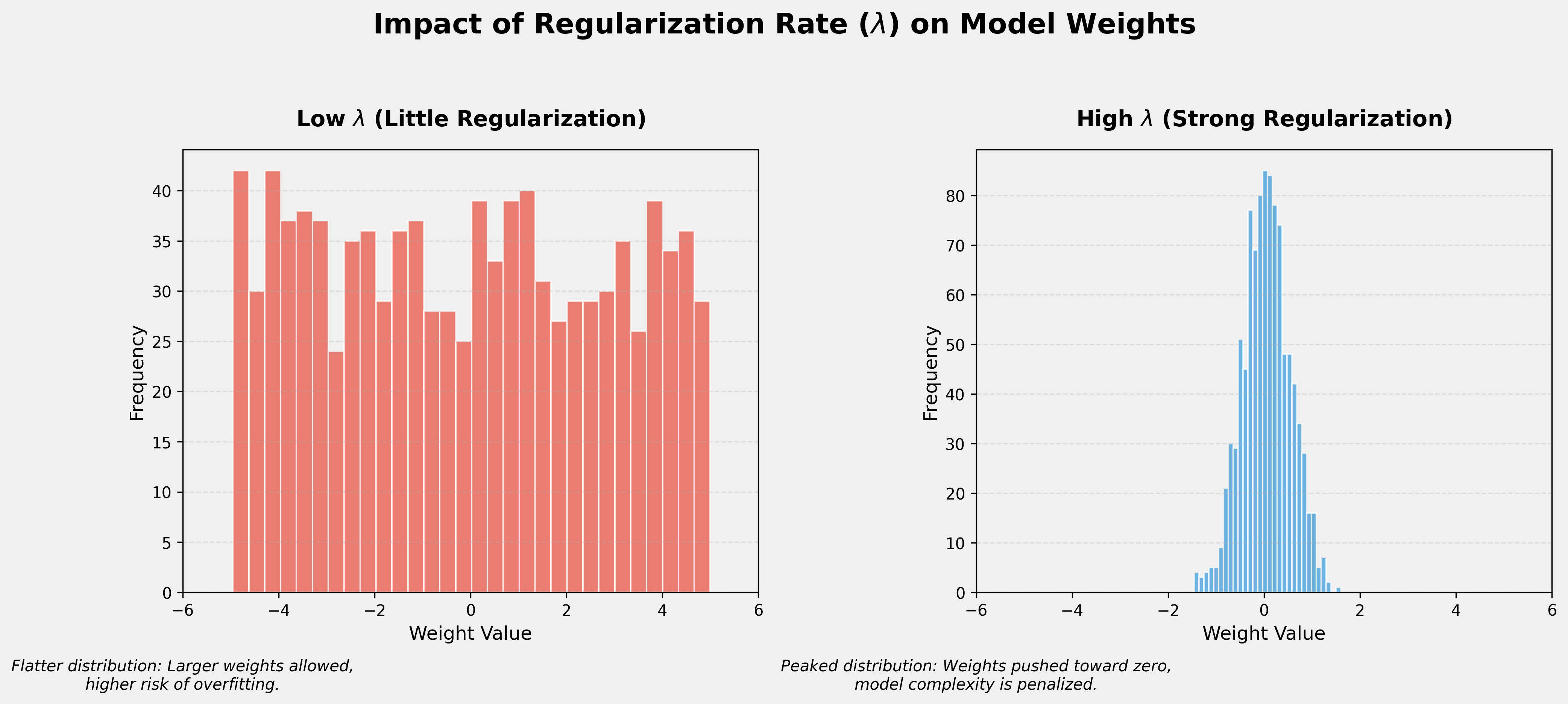
The regularization rate, lambda (), is a scalar that controls the balance between fitting the data and keeping the model simple.
- High : Penalizes large weights heavily. This forces most weights to be very small (near zero), creating a "simpler" model that is less likely to overfit but may underfit if too high.
- Low : Has a weaker effect on complexity. The model is allowed to have larger weights to minimize the training loss, which increases the risk of overfitting.
- : Regularization is disabled entirely.
Intuition: Squaring the Weights
By squaring the weights, L2 regularization penalizes "outlier" weights much more than small weights. This encourages the model to distribute its "importance" across many features rather than relying on just one or two.
Example: Simplifying a Complex Model Consider a model with six weights. Notice how one large weight dominates the complexity:
| Weight | Value | Squared () | % of Total Complexity |
|---|---|---|---|
| 0.2 | 0.04 | ~0.1% | |
| -0.5 | 0.25 | ~0.9% | |
| 5.0 | 25.0 | ~93.2% | |
| -1.2 | 1.44 | ~5.4% | |
| 0.3 | 0.09 | ~0.3% | |
| -0.1 | 0.01 | ~0.1% | |
| Total | 26.83 | 100% |
In this scenario, accounts for over 93% of the model's complexity. When L2 regularization is applied, the optimization algorithm will aggressively try to reduce the magnitude of to lower the overall penalty, forcing the model to find a more balanced solution.
(Example adapted from the Google Machine Learning Crash Course.)
Key characteristics of L2:
- Weight Decay: It discourages weights from becoming too large by penalizing them quadratically.
- Stability: It is effective at stabilizing weights, especially when there is high correlation (multicollinearity) between input features.
- Optimization: In PyTorch and other frameworks, this is often implemented as weight decay in the optimizer.
# Add L2 regularization (weight_decay) to the optimizer
optimizer = torch.optim.Adam(model.parameters(), lr=0.001, weight_decay=1e-5)
Comparison: L1 vs. L2
| Feature | L1 (Lasso) | L2 (Ridge) |
|---|---|---|
| Penalty | Sum of absolute weights () | Sum of squared weights () |
| Weights | Can be pushed to exactly zero | Become very small but not zero |
| Effect | Sparse solution / Feature selection | Small weights / General stabilization |
| Robustness | Robust to outliers | Less robust to outliers |
Dropout
Dropout is a simple yet powerful regularization technique specifically designed for neural networks. During training, it randomly "drops out" (i.e., sets to zero) a fraction of the neurons in a layer at each update step.
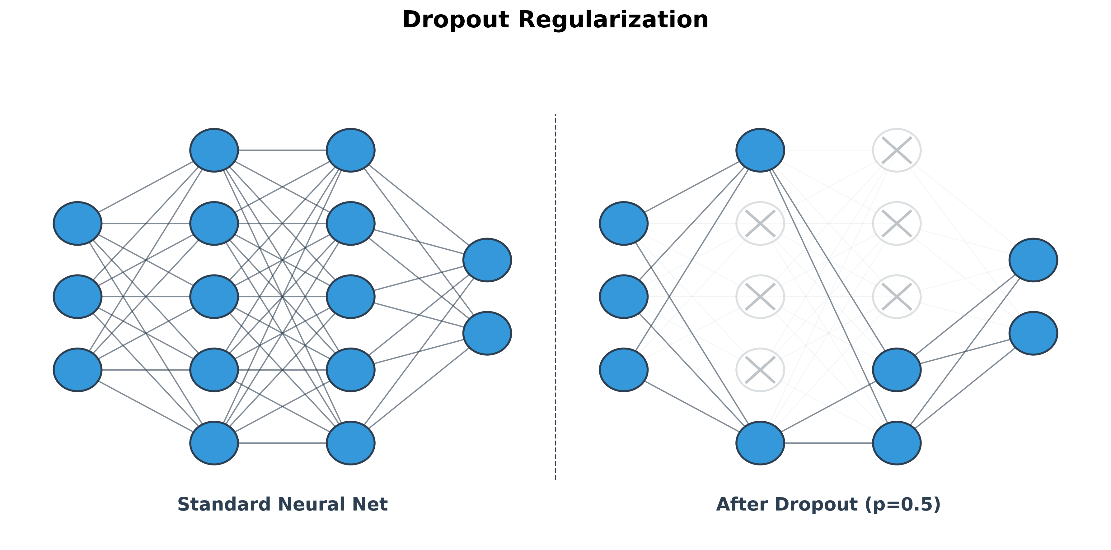
This has two main effects:
- It prevents neurons from co-adapting too much. Since a neuron's inputs can randomly disappear, it must learn to be more robust and not rely on any single input.
- It's like training a large ensemble of different neural networks. Each training step uses a different "thinned" network, and the final model is an average of all these networks.
Dropout is only applied during training. During testing or inference, the full network is used, but the outputs of the dropout layers are scaled down to account for the fact that more neurons are active.
In PyTorch, you can add a nn.Dropout layer to your model:
model = nn.Sequential(
    nn.Linear(input_size, hidden_size),
    nn.ReLU(),
    nn.Dropout(p=0.5),  # p is the probability of a neuron being dropped
    nn.Linear(hidden_size, output_size),
)
It is crucial to call model.train() before training and model.eval() before evaluation to ensure dropout is enabled and disabled correctly.
Early Stopping
Early Stopping is a more pragmatic form of regularization. The idea is to monitor the model's performance on a validation set (a portion of the training data held out from training) during the training process.
You continue training as long as the performance on the validation set is improving. As soon as the validation performance starts to get worse, you stop training. The point at which you stop is the point where the model has started to overfit the training data. The model's parameters from that point are then saved as the final model.
This technique is effective and easy to implement, preventing the model from training for too many epochs and overfitting.