Data Transformations
There are a few other functions and techniques that you should know that come in handy when transforming data from one form to another to derive better insights. In this lesson, you will learn a few of these techniques.
Segmentation
Segmentation is a widely used technique in data analysis. For categorical data, the data is already segmented, but for continuous numerical data, you will have to come up with your own formula. Using the segmentation (or binning) technique, you can categorize or discretize a given continuous variable for analysis.
As an example, let's look at the age column of the Titanic data. We have a wide range of travelers, from 0.42-year-old babies to 80-year-old senior citizens. One possible segmentation is to bucket the travelers into 'children' (below the age of 13), 'teenagers' (travelers between 13 and 19 years old), 'adults' (from 20 to 60 years old), and beyond 60, we will label them as 'seniors'. Pandas provides a built-in function, cut, to accomplish this task easily. This function returns a new Series object that will have the categorical values based on our segmentation. We can then attach this Series as another column to our original DataFrame, thereby making it part of the data. Let's do that:
import numpy as np
import pandas as pd

titanic_df = pd.read_csv(
    "https://raw.githubusercontent.com/jravi123/datasets/refs/heads/main/titanic.csv"
)
segments = [-1, 12, 19, 60, np.inf]
labels = ["child", "teenager", "adult", "senior"]
age_group = pd.cut(titanic_df.age, bins=segments, labels=labels)
titanic_df["age_group"] = age_group
titanic_df.head(3)
Output:
   survived  pclass     sex   age  sibsp  parch     fare embarked  class
0         0       3    male  22.0      1      0   7.2500        S  Third
1         1       1  female  38.0      1      0  71.2833        C  First
2         1       3  female  26.0      0      0   7.9250        S  Third

     who  adult_male deck  embark_town alive  alone age_group
0    man        True  NaN  Southampton    no  False     adult
1  woman       False    C    Cherbourg   yes  False     adult
2  woman       False  NaN  Southampton   yes   True     adult
In the code above, the first line declares the segments with the boundaries. The first array element will be taken as the min value for the first segment, and the second element will be considered the max value. The second segment will consider the second element as the min value and the third element as its max value, and so on for the third and last segments. Notice that the last segment has an upper max value of infinity, which is declared by using np.inf.
Note: The reason we start from -1 and not 0 is to include all values that are '0', as the range starts from the value above the declared min value.
The second line initializes the list of labels for our segments. The third line is where we use the cut function, which takes in the column values that need to be categorized, along with the two arrays for specifying the segments and labels. This function returns a Series object. Then, in the last line, we add the new column to our DataFrame by just defining the new column name and attaching the Series returned by cut. That's it!
When you see the first three rows of your new DataFrame, you will notice that a new column, 'age_group', has been added to the original, thereby successfully converting continuous numerical data to categorical data, ready for deeper analysis. By default, new columns are inserted at the end. Note that the number of values for the new column should match the number of rows, or it can be a single scalar value, in which case the value is broadcast to all rows.
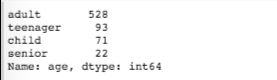
You can get the frequency of the bin labels by using the value_counts() function, as shown below:
pd.value_counts(age_group)
Another way of applying value_counts is shown below:
titanic_df["embark_town"].value_counts()
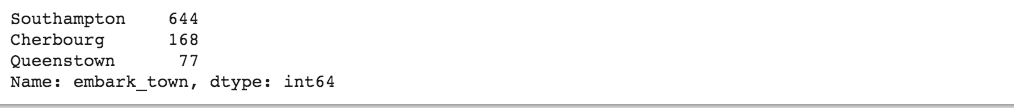
value_counts returns the frequency counts in descending order.
There are many other arguments you can add and set for the cut function. Refer to the documentation:
http://pandas.pydata.org/pandas-docs/version/0.22/generated/pandas.cut.html
** qcut function **
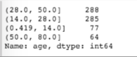
You can also segment your data using quantiles as boundaries by using the qcut function. Let's see what the segmented counts are if we do this at the 10, 50, and 90 quantiles. Here is an example:
quantiles = pd.qcut(titanic_df["age"], [0, 0.1, 0.5, 0.9, 1.0])
pd.value_counts(quantiles)
You can also just provide the number of buckets instead of specifying the quantiles. You can also specify labels.
Official reference on qcut: https://pandas.pydata.org/pandas-docs/stable/reference/api/pandas.qcut.html
Using the Map Function
You can apply a map function to individual field values and create a new column. Suppose you want to map the various
cities to the countries from where people embarked on the titanic_df. You would create a dictionary with city-to-country entries
and then apply this mapping to the individual values of the city column using the map function. Here is the code:
city_to_country = {
"Southampton": "Great Britain",
"Cherbourg": "France",
"Queenstown": "Great Britain",
}
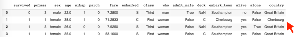
titanic_df["country"] = titanic_df["embark_town"].map(city_to_country)
titanic_df
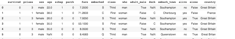
From the results, you can see that a new column, 'country', has been added, which is derived from applying the map to the individual column values of the 'embark_town' column. Note that while this example uses a dictionary, you could also use a Series object, with the index being the key values of the dictionary shown above.
** Using the replace function**
You can also use replace in place of map above. Here are the same results obtained using replace:
city_to_country = {
    "Southampton": "Great Britain",
    "Cherbourg": "France",
    "Queenstown": "Great Britain",
}

titanic_df["country"] = titanic_df["embark_town"].replace(city_to_country)
titanic_df
However, note the difference: if the city_to_country map has a missing value, the map function adds a NaN value, but in the case of replace, it fills in the original column value as-is. Here is an example in which one map value is missing:
city_to_country = {"Southampton": "Great Britain", "Queenstown": "Great Britain"}

titanic_df["country"] = titanic_df["embark_town"].replace(city_to_country)
titanic_df
city_to_country = {"Southampton": "Great Britain", "Queenstown": "Great Britain"}

titanic_df["country"] = titanic_df["embark_town"].map(city_to_country)
titanic_df
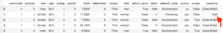
Note that you can also just replace some values in the existing column by providing one or more map values.
Using the shift() function
You can use the shift() function to move a row or column by the desired number of index positions. This function takes a scalar parameter called periods, which represents the number of shifts for the desired axis.
Let's take an example of data showing the total number of infections of a disease tabulated for a few days.
df = pd.DataFrame(
    {
        "date": ["01/01/2020", "01/02/2020", "01/03/2020", "01/04/2020"],
        "total_infections": [49, 55, 77, 99],
    }
)

df.shift(1)
	date	total_infections
0	NaN	            NaN
1	01/01/2020          49.0
2	01/02/2020	    55.0
3	01/03/2020	    77.0
You can fill a default value for the shifted row by adding the fill_value argument.
If you want to have another column that shows the previous day's count next to the present day's count, you could use shift() on the column instead of the entire DataFrame. Here is an example:
df["prev_day"] = df["total_infections"].shift(1, fill_value=0)

df
            date    total_infections	prev_day
0	    01/01/2020	    49	            0
1	    01/02/2020	    55	            49
2	    01/03/2020	    77	            55
3	    01/04/2020	    99	            77
Now you can add another column that computes the average rate of change in infection for three days, as shown below.
Note: The date column should have sorted values; otherwise, your calculations will be incorrect. If the dates are not sorted, you can sort them using the expression below:
df.sort_values(by=['date'], inplace=True)
You can also make the index a time series by setting the date column to be the index.
Then you can sort the index using the df.sort_index() method.
At that point, you can also apply a lot of time series-related functions that you will explore in Chapter 5.
df["3_day_average"] = (
    df["total_infections"]
    + df["total_infections"].shift(1, fill_value=0)
    + df["total_infections"].shift(2, fill_value=0)
) / 3

df
    date	    total_infections	3_day_average
0	01/01/2020	    49	            16.333333
1	01/02/2020	    55	            34.666667
2	01/03/2020	    77	            60.333333
3	01/04/2020	    99	            77.000000
mask() method
The mask() method can be used in place of complex conditional statements to achieve the same end result. Here is an example of flipping all values less than 60 to "Fail".
df = pd.DataFrame(
    {
        "marks": [70, 55, 100, 88],
        "age": [29, 32, 31, 28],
        "sex": ["F", "M", "F", "F"],
        "name": ["Jane", "John", "Sally", "Sandy"],
        "ssn": ["1234", "3456", "4567", "5678"],
    }
)
df["marks"].mask(df["marks"] < 60, "Fail", inplace=True)
df
      marks	age	sex	name	ssn
0	70	29	F	Jane	1234
1	Fail	32	M	John	3456
2	100	31	F	Sally	4567
3	88	28	F	Sandy	5678
You can apply this function at the DataFrame level as well to apply it to all rows and columns, although the example shown above is for checking the condition on one column.