Date and Time

Date and/or time are fundamental data points in many domains, like stock price analytics, IoT sensor data analytics, etc. In Python, we use the datetime module for the most part. If you have followed our eBook on Python, you would have played with the datetime and time modules: https://ebooks.mobibootcamp.com/python/datetime.html

While the Python modules for dates are good for creating one-time, individual date objects, there are no built-in structures for handling large arrays of dates. In data analytics, we predominantly use collections of dates and rarely use a single date object. That is when NumPy's datetime64 data type comes to our rescue. datetime64 provides array support for datetime functionality, along with supporting many common date formats right off the bat.

The Pandas library makes use of NumPy's datetime structures, datetime64 and timedelta64 dtypes, along with structures in the dateutil package, and also uses a large number of structures from other Python libraries like scikits.timeseries. The Pandas package has also created new functionality for manipulating time series data.

dateutil package

When you install Pandas or Anaconda, the dateutil package is also installed. This package provides a very handy parser that eliminates the need to use the strptime datetime method. Recall the date parsing shown using the Python datetime module at https://ebooks.mobibootcamp.com/python/datetime.html

Here is a date parsing example using dateutil that simplifies the task:

from dateutil.parser import parse

print(type(parse("2018-01-31")))
print(parse("Jan 31, 2018 11:45 AM"))

# In many locales around the world,
# the day appears before the month in a date representation, so pass dayfirst=True
print(parse("1/12/2018", dayfirst=True))

Output:
<class 'datetime.datetime'>
2018-01-31 11:45:00
2018-12-01 00:00:00

As you can see from the example above, using the parse function from dateutil simplifies date parsing, as many standard date formats are automatically identified and parsed. Pandas uses this parser when reading files into a DataFrame, which is explained in the next sections in detail.

Pandas Date/Time

By using all the modules explained above, Pandas has exposed two convenient date/time structures that can be used with Series and DataFrames, the two main building blocks of Pandas.

• Timestamp: Pandas has a structure called Timestamp, which is essentially a replacement for Python's datetime and is interchangeable with it in most cases. Pandas stores timestamps using NumPy’s datetime64 data type at nanosecond resolution.

• DatetimeIndex: The Pandas DatetimeIndex is used to create an index of Timestamp types. This can work as an index for both Series and DataFrames.

Note, however, that you can set a datetime type object to a DatetimeIndex, and they are automatically converted to Timestamp. You really do not have to do anything extra to get a Timestamp. A Series with Timestamp/datetime values as its index will become a DatetimeIndex under the hood.

Timeseries

A Series object made of contiguous Timestamp-related data as its index is a time series. The series could be just dates without time, or with both date and time. Time series data are prevalent in finance/economics (stock prices over time, company turnover on a monthly or weekly basis, etc.), in biology (how diseases spread over time, multivariate observations of molecules and proteins over time, etc.), in Physics (speed/acceleration over time, etc.), in companies (customer's usage data, log data), etc.

There is nothing as simple and elegant as a line chart. A line chart displays information as a series of data points connected by a line segment. A line chart is the de facto standard for showing time series data.

Weekly Demolition Count

In Pandas, you can slice, aggregate, and chart time series data just like any other numerical data that we have worked with so far.

Plotting time series data

Once you have the index of a Series or DataFrame made up of the Timestamp data type, it is very easy to plot a line graph. Here is an example:

import pandas as pd
import matplotlib.pyplot as plt

# Read data
detroit_demolitions = pd.read_csv(
    "https://raw.githubusercontent.com/jravi123/datasets/refs/heads/main/datasets/Detroit_Demolitions_withColumns.csv",
    parse_dates=[4],
)

# for column names, replace space with an underscore and also change the case to lower
detroit_demolitions.columns = detroit_demolitions.columns.str.replace(
    " ", "_"
).str.lower()

# strip $ symbol and convert the type to float for 'price' column
# Regex is safer for removing $
detroit_demolitions["price"] = (
    detroit_demolitions["price"].replace({"\$": "", ",": ""}, regex=True).astype(float)
)

# Get a timeseries to plot
ts = pd.Series(
    detroit_demolitions["price"].values, index=detroit_demolitions["demolition_date"]
)
ts = ts.sort_index()

# Plot
plt.figure(figsize=(12, 6))
plt.plot(ts.index, ts.values, color="#3498db", alpha=0.6)
plt.title("Demolition Prices Over Time")
plt.xlabel("Demolition Date")
plt.ylabel("Price ($)")
plt.show()

In the example above, after all the cleaning steps, you create a new Series object with two columns: 'price' and 'demolition_date'. The index of this Series object is set with the values from the 'demolition_date' column. Then, by invoking the plot() method on the Series object, you get a line graph of prices vs. date.

Note, however, that you can also plot by directly using the column from the DataFrame. You will see those examples in the stock price plots below.

Now, run the statement below and see what is printed out:

ts.index

Did you create a DatetimeIndex type? No, but your datetime column Series is automatically converted to a DatetimeIndex behind the scenes.

You can also select a particular index by passing the date as a string, as shown below:

ts['2016-03-08']

Output:

Now you can see that there were many demolitions on March 8th. So, the index is not unique, as there are many duplicates, and that is allowed.

You can, in fact, provide the selection in any standard format, and it will be parsed to get the correct selection. Try the statement below, and you will still see the same result:

ts['03/08/2016']

Output:

You can also input just the year, and all the entries for that year will be selected:

ts['2016']

Output: Not shown to keep it concise, but we encourage you to try it on your machine.

You can also perform a range query:

ts['1/6/2017':'1/11/2017']

Output: Not shown to keep it concise, but we encourage you to try it on your machine.

Now that we see that the indexes have duplicates, we can even groupby on the date by passing level=0 (which stands for the one index that we have). In the case of MultiIndex scenarios, you would choose a level other than 0.

ts.groupby(level=0).count()

Output: Not shown to keep it concise, but we encourage you to try it on your machine.

In place of count, you could also use mean() or sum(), and accordingly, the 'price' will be summed or averaged.

Resampling and Frequency Conversion

While the plot above is against all the dates in the dataset, sometimes you may want to find monthly, weekly, or yearly aggregations instead of every date entry. You may even want to aggregate based on the date itself. Now that we know that every date has many demolitions, you may want to aggregate the total price for every day and then plot that graph. The process of converting a time series from one frequency to another is called resampling.

In resampling, there are two commonly used scenarios:

• Downsampling: Changing higher-frequency data to lower-frequency data. E.g., converting daily or weekly frequency data to monthly, quarterly, yearly, etc.
• Upsampling: Changing lower-frequency data to higher-frequency data. E.g., converting monthly frequency data to daily, weekly, etc.

You use the resample() method on Pandas to get these conversions. Below is an example of converting the daily frequency data referenced above to a monthly frequency:

ts2 = ts.resample("ME").sum()  # 'ME' is Month End
print(ts2)

plt.figure(figsize=(12, 6))
ax = ts2.plot(color="#9b59b6", marker="s")
plt.title("Total Monthly Demolition Cost")
plt.xlabel("Date")
plt.ylabel("Total Cost ($)")


# Format Y axis to Millions for readability
def millions(x, pos):
    return "$%1.1fM" % (x * 1e-6)


ax.yaxis.set_major_formatter(plt.FuncFormatter(millions))
plt.show()

'ME' stands for monthly end frequency. Notice that the y_ticklabels are formatted to show "Millions" (M) to avoid scientific notation.

Official reference

You can also select only 2017 data if you want and aggregate it on a monthly basis by running the statement below:

ts2 = ts["2017"].resample("ME").sum()
plt.figure(figsize=(12, 6))
ts2.plot(color="#2ecc71", marker="o", linewidth=2.5)
plt.title("Total Demolition Cost in 2017 (Monthly)")
plt.ylabel("Total Cost ($)")
plt.show()

Exercise:

1. Resample to Quarterly and Yearly with price aggregation and plot the graph.

Parsing Dates With DataFrames

When it comes to parsing a date to a Timestamp from a string value in a dataset, there are a few options:

to_datetime method of DataFrame

In the example below, you will first read the CSV file from Google storage and then parse the date column.

import pandas as pd

detroit_demolitions = pd.read_csv(
    "https://raw.githubusercontent.com/jravi123/datasets/refs/heads/main/datasets/Detroit_Demolitions_withColumns.csv"
)
print(detroit_demolitions.info())
print(detroit_demolitions.head(1))

Output:

<class 'pandas.core.frame.DataFrame'>
RangeIndex: 12227 entries, 0 to 12226
Data columns (total 11 columns):
Address 12227 non-null object
:
Demolition Date 12227 non-null object
:

||

From the output above, you can notice that the Demolition Date column is of object type. Using the type() command, you will see that the value is a string type.

type(detroit_demolitions["Demolition Date"][0])

Output:
str

Now you can convert this string to a Pandas Timestamp using the to_datetime() method by specifying the format of the string date. If you see in the output above, the date is in the mm/dd/yyyy format, so using the formatter below, you can convert the string to a date type.

detroit_demolitions["Demolition Date"] = pd.to_datetime(
    detroit_demolitions["Demolition Date"], format="%m/%d/%Y"
)

As the date string is in one of the standard formats, you can skip providing the format argument in the example above. However, it is good practice to provide this argument to ensure that dates are not erroneously parsed when the date string is in a non-standard format.

parse_dates argument

However, there is a more elegant solution to the problem above. You can use the parse_dates argument to convert the string to a Timestamp while reading the CSV file. Below is the shortened code to perform the same task:

detroit_demolitions = pd.read_csv(
    "https://raw.githubusercontent.com/jravi123/datasets/refs/heads/main/datasets/Detroit_Demolitions_withColumns.csv",
    parse_dates=[4],
)
print(detroit_demolitions.info())

Output:

<class 'pandas.core.frame.DataFrame'>
RangeIndex: 12227 entries, 0 to 12226
Data columns (total 11 columns):
Address 12227 non-null object
:
Price 12227 non-null object
Demolition Date 12227 non-null datetime64[ns]
:

In the code above, you set the argument parse_dates with the column number to apply the default parser. Since the date is the 5th column in our dataset, you see [4] as the column number. Notice that we did not pass any formatter in this implementation. That is because the date string is in a standard format, and the default parser will suffice.

However, if you have a date string in a non-standard format, you can pass your own parser function to use for date conversion. Here is an example:

from datetime import datetime

parser = lambda mydate: datetime.strptime(mydate, "%m/%d/%Y")
pd.read_csv(
    "https://raw.githubusercontent.com/jravi123/datasets/refs/heads/main/datasets/Detroit_Demolitions_withColumns.csv",
    parse_dates=[4],
    date_parser=parser,
)

Although creating a parser for the example above is moot and not required, as the default parser is able to do the job for the given string format, in the case of a non-standard date string, you can create a custom parser as shown above.

Using the astype method

You can also use the astype method to convert string values to the NumPy datetime64 type. An example is shown below:

df = pd.DataFrame({"date": ["2018-01-04", "2020-05-03"]})
df = df.astype({"date": "datetime64[ns]"})
df.info()

Official reference

Moving window functions

The rolling operator resembles resample and groupby and can be called on a Series or DataFrame. You pass the window argument, which is expressed as the number of periods, which enables grouping over the period passed as an argument. In the example below, the sliding window period is 100. A sliding window is useful for smoothing noisy or gappy data. Of course, you can change that 100 to any number of periods over which you want to find the average. The bigger the window, the bigger the smoothing effect you will see. The smallest window resembles the daily price plot itself.

import pandas as pd
import matplotlib.pyplot as plt

df = pd.read_csv(
    "https://raw.githubusercontent.com/jravi123/datasets/refs/heads/main/datasets/HistoricalQuotes%20AMZN.csv",
    parse_dates=True,
    index_col="date",
)
# Clean data
for col in df.columns:
    if df[col].dtype == "object":
        df[col] = df[col].str.replace(",", "").astype(float)

df = df.sort_index()

plt.figure(figsize=(12, 6))
df.open.plot(label="Daily Open Price", alpha=0.5, color="gray")
df.open.rolling(100).mean().plot(
    label="100-Day Moving Avg", color="#e74c3c", linewidth=2.5
)
plt.title("AMZN Closing Price vs 100-Day Moving Average")
plt.legend()
plt.show()

By default, rolling functions require all of the values in the window to be valid. That is why you see that the rolling window plot starts later than the daily price plot.

Below, you can see an example with min_periods set to 10. Here, we calculate the standard deviation for the window period. We plot it on a secondary axis to see the volatility clearly.

plt.figure(figsize=(12, 6))
ax1 = df.open.plot(label="Price", alpha=0.5, color="gray")
plt.ylabel("Price ($)")

ax2 = ax1.twinx()
df.open.rolling(200, min_periods=10).std().plot(
    ax=ax2, label="Rolling Std", color="#d35400", linewidth=2
)
plt.ylabel("Rolling Std Deviation")
plt.title("AMZN Price Volatility (Rolling Standard Deviation)")
plt.legend(loc="upper left")
plt.show()

Annotations in Matplotlib

You can add annotations with text and arrows to highlight certain important points in your charts. You can even add just text to show some important messages. Both of these are applied to the subplot object. Here is an example in which we first get a handle on the subplot ax, and then use the annotate and text functions to add an annotation and text, respectively.

from datetime import datetime

plt.figure(figsize=(12, 6))
ax = df.open.plot(color="#2980b9")

# Define annotation point (2016 Election)
x_point = datetime(2016, 11, 4)
# Get Y value safely
y_point = df.asof(x_point)["open"]

ax.annotate(
    "2016 Election",
    xy=(x_point, y_point),
    xytext=(x_point, y_point + 200),
    arrowprops=dict(facecolor="black", shrink=0.05),
    ha="center",
    fontsize=12,
    fontweight="bold",
    bbox=dict(boxstyle="round,pad=0.3", fc="white", ec="black", alpha=0.8),
)

# Add text for rally
ax.text(
    datetime(2017, 5, 1),
    y_point + 50,
    "Post-Election Rally \u279c",
    fontsize=12,
    color="#27ae60",
    fontweight="bold",
    ha="left",
)

# Zoom to a certain x and y range
ax.set_xlim(datetime(2016, 1, 1), datetime(2018, 1, 1))
ax.set_ylim(400, 1300)
plt.title("AMZN Stock Analysis: 2016 Election Impact")
plt.show()

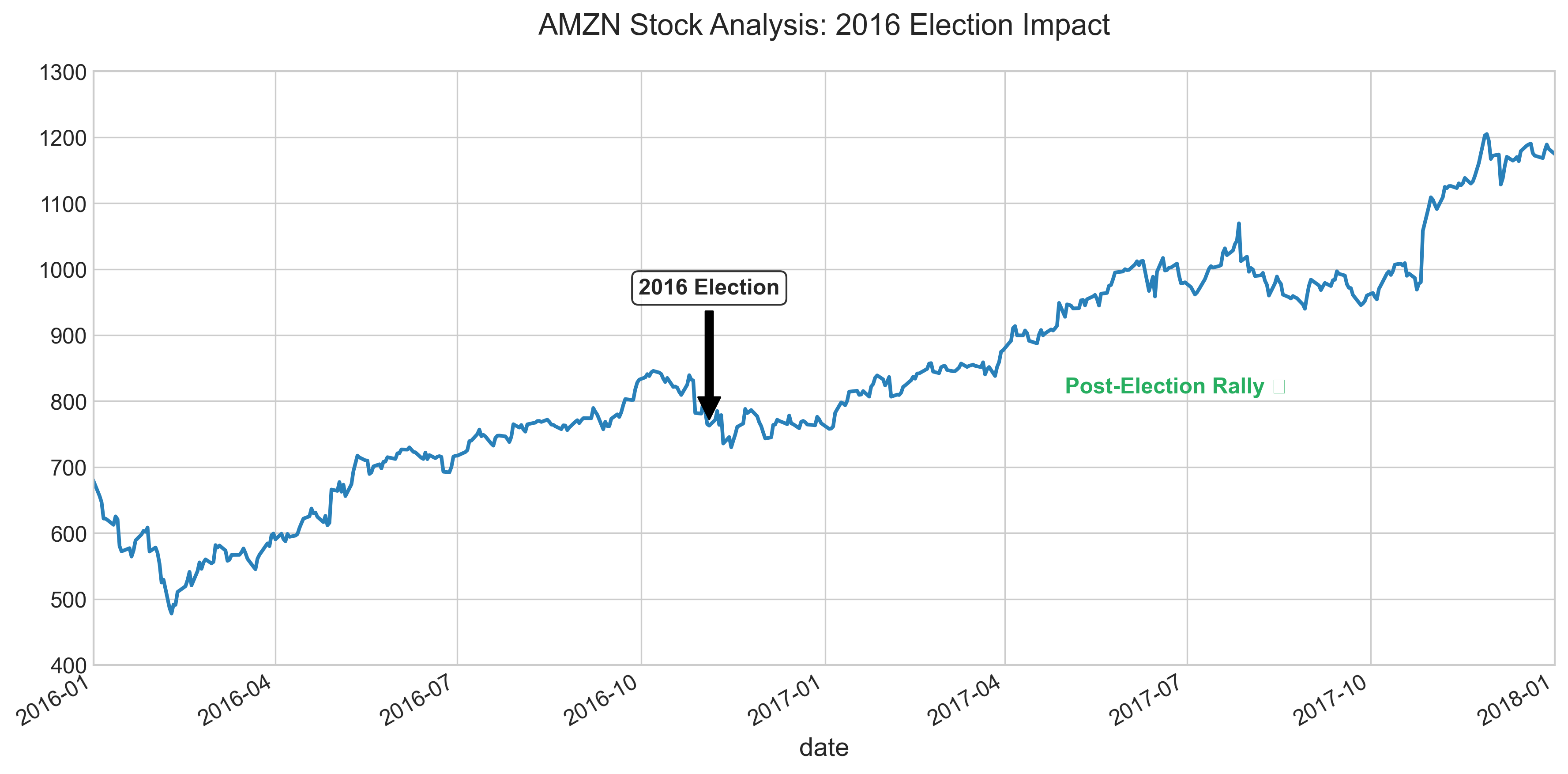
In the annotate method, the xy point is the point of annotation, and if the optional xytext is given, the text will be added at the given x and y point. The line length will be computed automatically by taking the distance between the annotation point and the annotation text. Setting xlim and ylim allows you to zoom in to a specific portion of the chart.

There are many other optional attributes, and the full reference is here: https://matplotlib.org/api/_as_gen/matplotlib.pyplot.annotate.html

The text function takes the x-value, y-value, and the value of the text to be displayed. Here also, there are other optional attributes you can set.

Reference: https://matplotlib.org/api/_as_gen/matplotlib.pyplot.text.html

Remote Data Into Pandas

You can directly get data from many different remote sources, mostly connected with financial and ticker symbols, using the Pandas datareader library.

Refer to this link to learn more: https://pydata.github.io/pandas-datareader/remote_data.html