Regression

Regression is a statistical method that attempts to determine a relationship between one dependent variable (the target, y) and one or more independent variables (the features, X). The goal is to build a model that can predict a continuous numerical value.

The model, or function f(X), is built using training data. Once trained, the model can be used to predict the y value for new, unseen X values.

Linear Regression

The simplest form of regression is Linear Regression, which assumes that the relationship between the dependent and independent variables is linear.

Univariate Linear Regression

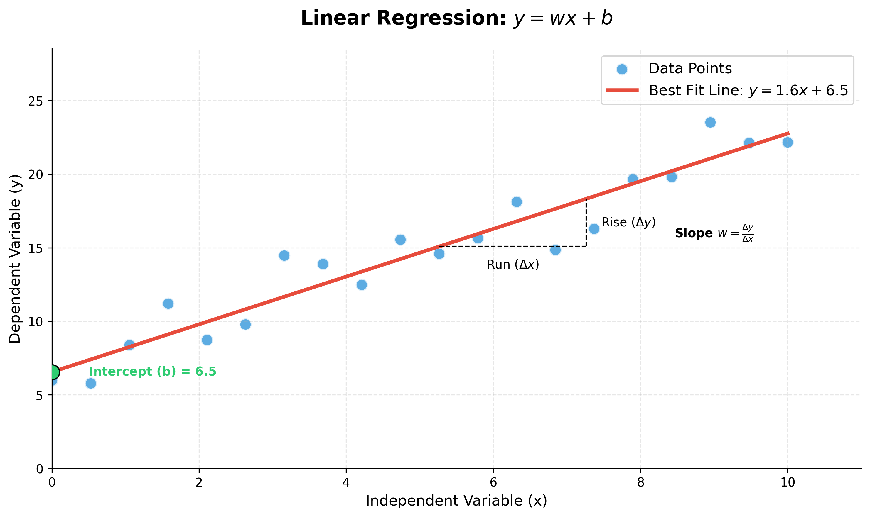
When there is only one independent variable (x), the formula is a simple line:

y = wx + b

In this equation:

• y is the dependent variable we are trying to predict.
• x is the independent variable.
• w is the coefficient (or weight), representing the slope of the line. It tells us how much y changes for a one-unit change in x.
• b is the intercept (or bias term), representing the value of y when x is 0.

(Note: The term 'bias' here is different from the 'bias' in the bias-variance tradeoff. Here, it's simply part of the linear equation.)

Finding the Best-Fitting Line

The goal of training a linear regression model is to find the optimal values for the coefficient w and the intercept b that result in the "best-fitting line" for the data.

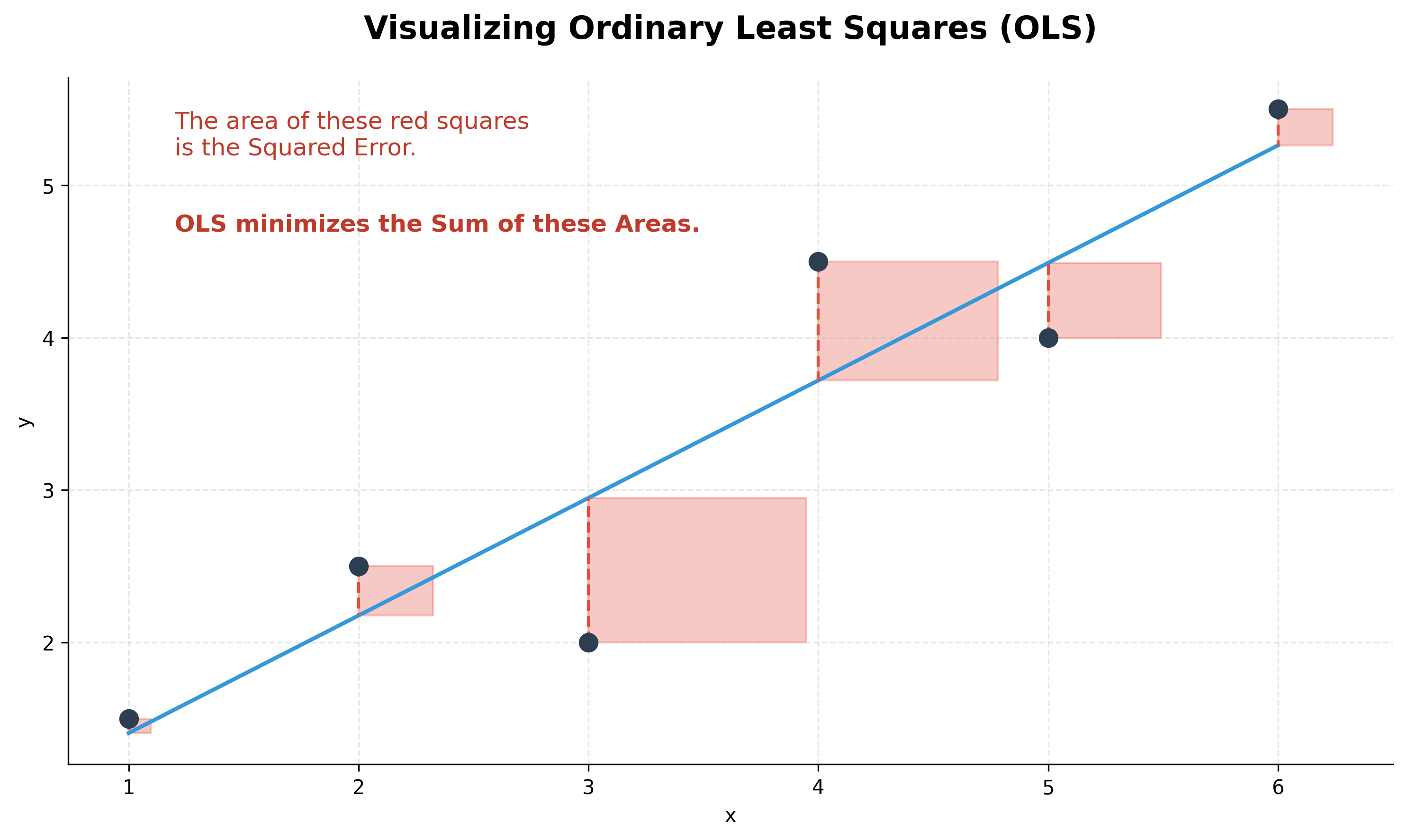
To find this line, the most common method is Ordinary Least Squares (OLS). The core idea is to minimize the Sum of Squared Errors (SSE). For each data point, we calculate the vertical distance between the actual value (y) and the predicted value on the line (ŷ). This distance is the error. We square each error (to make them all positive) and sum them up. The OLS method finds the unique line that makes this total sum of squares as small as possible.

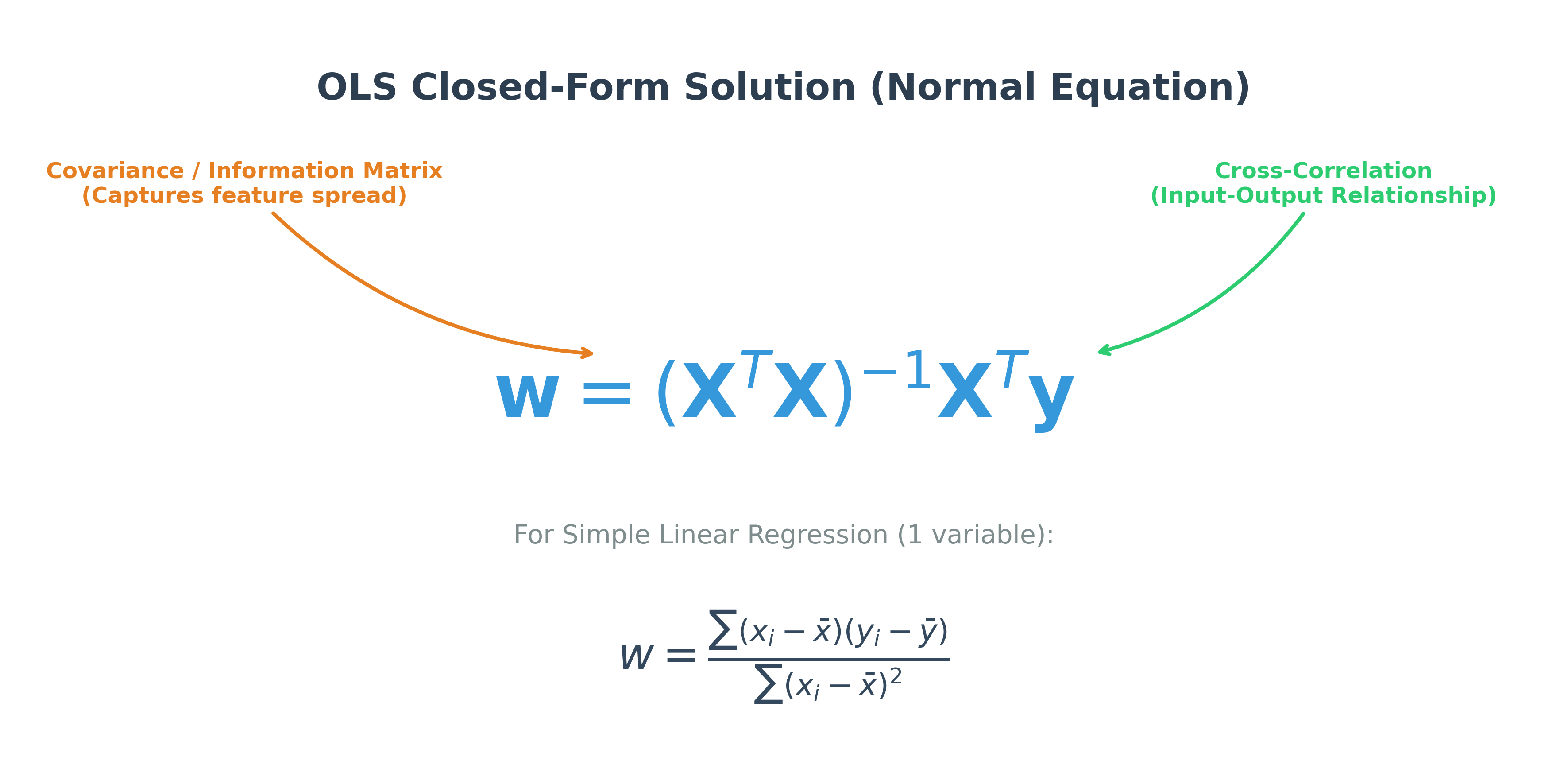
This optimization leads to a closed-form solution known as the Normal Equation, which allows us to calculate the optimal weights directly:

Multivariate Linear Regression

If the number of independent variables (features) is more than one, the model is a multivariate linear regression. The equation expands to include a coefficient for each feature:

y = w₁x₁ + w₂x₂ + ... + wₙxₙ + b

This is often simplified using vector notation:

y = wᵀ * x + b

Assumptions for Linear Regression

For a linear regression model to be accurate and reliable, several assumptions about the data should hold true:

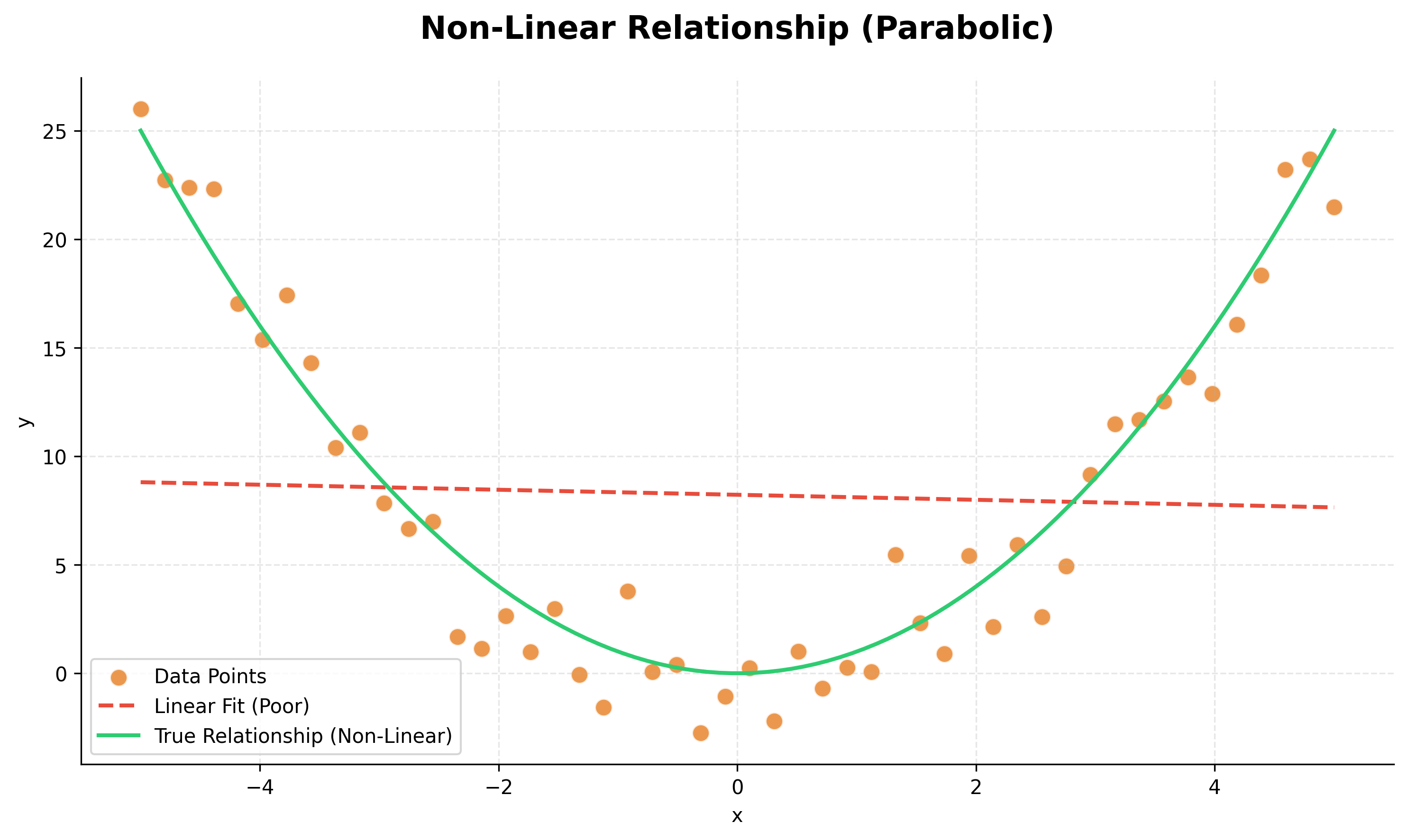
• Linearity: The relationship between the independent variables and the dependent variable should be linear.

• No Omitted Variable Bias (OVB): All relevant variables should be included in the model. Leaving out important variables can distort the coefficients of the included ones.

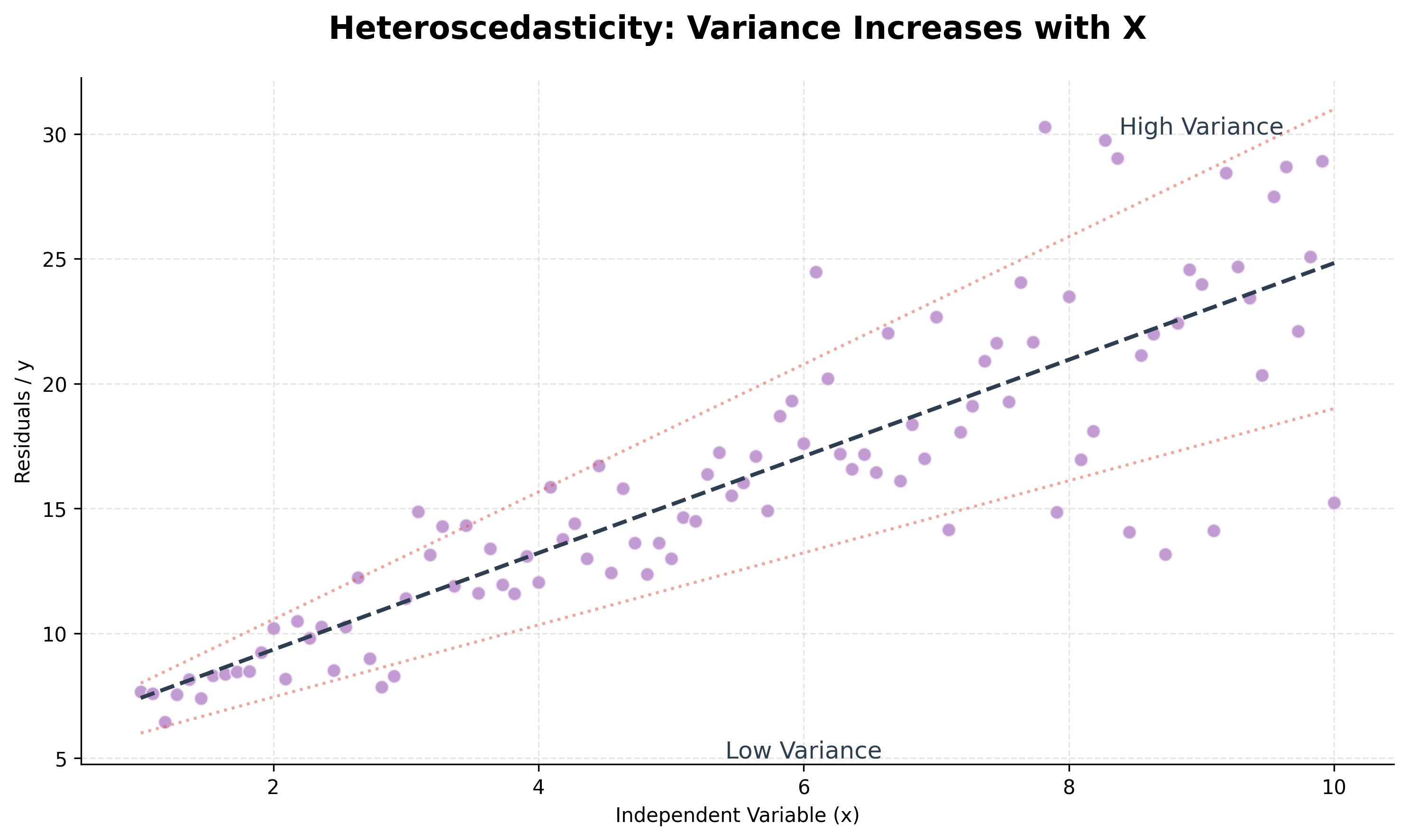
• Normality and Homoscedasticity of Errors: The errors (residuals) should be normally distributed. Homoscedasticity means the variance of the errors is constant across all levels of the independent variables. The opposite is heteroscedasticity, where the error variance changes.

  

• No Autocorrelation of Errors: The errors should be independent of each other.

• No Multicollinearity: The independent variables should not be highly correlated with each other.

From Regression to Classification

While regression is used to predict continuous values (like price or temperature), classification is used when the target variable is a category.

Examples of classification include:

• Classifying an email as 'spam' or 'not spam'.
• Classifying if a customer will 'default' or 'not default' on a loan.
• Classifying an image as a 'cat', 'dog', or 'elephant'.

Logistic Regression

Logistic Regression is a popular algorithm used for binary classification. Despite its name, it's a classification algorithm, not a regression one. It predicts the probability that an input belongs to a particular class (e.g., the probability of an email being spam).

Logistic regression works in two steps:

1. It calculates a score using a linear equation, just like linear regression: z = wᵀ * x + b
2. It then passes this score through a Sigmoid (or Logistic) function, which squashes the output to a value between 0 and 1. This value can be interpreted as a probability.

probability = σ(z) = 1 / (1 + e⁻ᶻ)

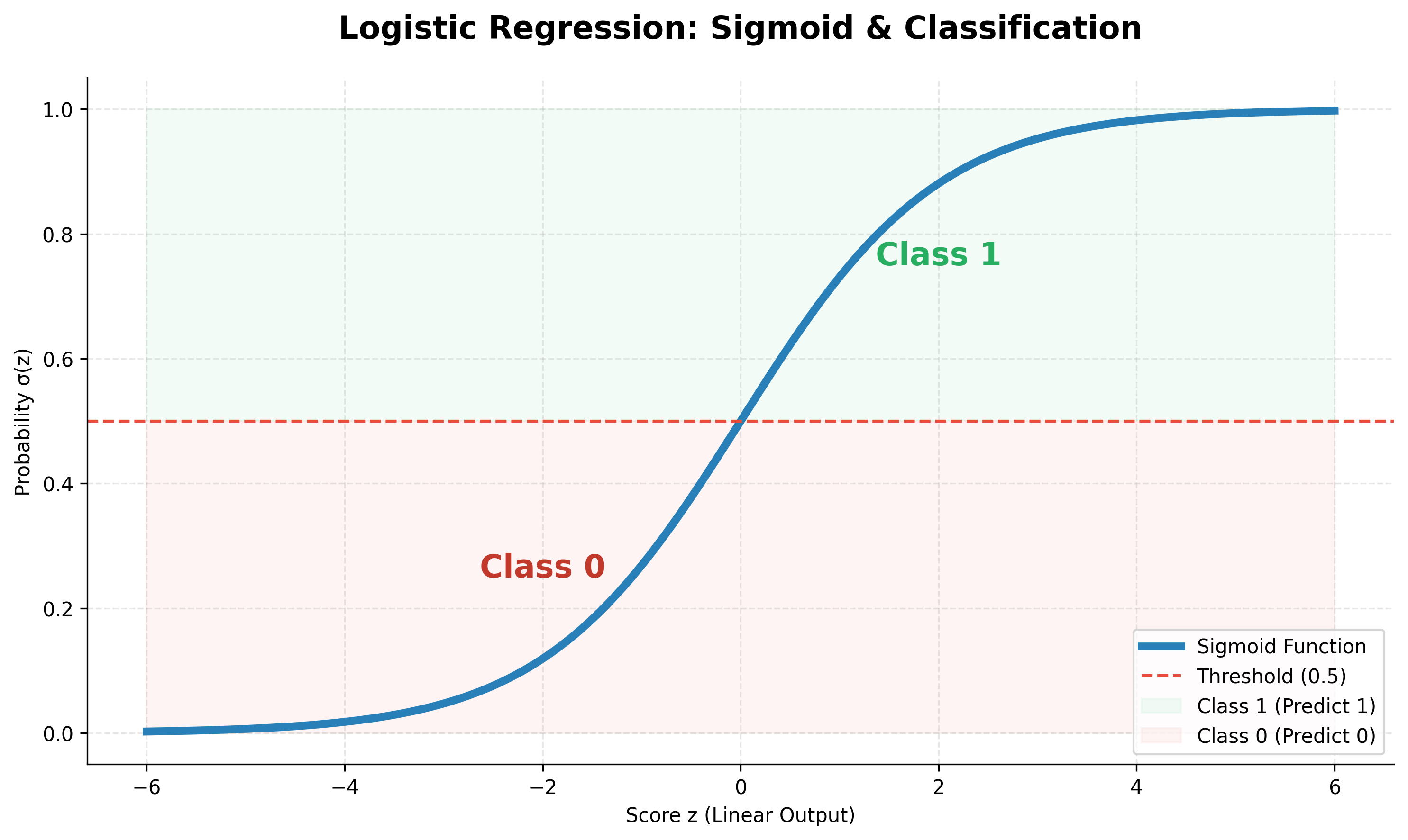
The output of the sigmoid function has these properties:

• If z is a large positive number, then σ(z) approaches 1.
• If z is a large negative number, then σ(z) approaches 0.
• If z = 0, then σ(z) = 0.5.

A threshold (typically 0.5) is then used to convert this probability into a class prediction. If the probability is > 0.5, the model predicts class 1; otherwise, it predicts class 0.

Multi-class Logistic Regression

For classification problems with more than two classes, an extension of the sigmoid function called the Softmax function is used. It calculates the probabilities for each class, ensuring that all probabilities sum to 1.

Other Algorithms for Regression and Classification

While linear and logistic regression are fundamental, many other algorithms can perform these tasks, often with higher accuracy. These include:

• Decision Trees
• Random Forest
• Gradient Boosting Machines (like XGBoost)

Most of these algorithms can be used for both classification and regression. They are covered in subsequent chapters.