Interactive Visualizations with Plotly Express
While Matplotlib and Seaborn are excellent for static publications, modern data exploration often requires interactivity—zooming, panning, hovering, and animating changes over time. Plotly Express is a high-level Python visualization library that makes creating complex, interactive charts incredibly simple.
Note on Interactivity: The visualizations shown on this page are static previews (PNG images). To experience the full interactivity—such as hovering for data details, clicking the animation slider, or zooming—you must run this code in a live Python environment like a Jupyter Notebook or Google Colab.
In this chapter, we will explore some stunning examples using standard datasets.
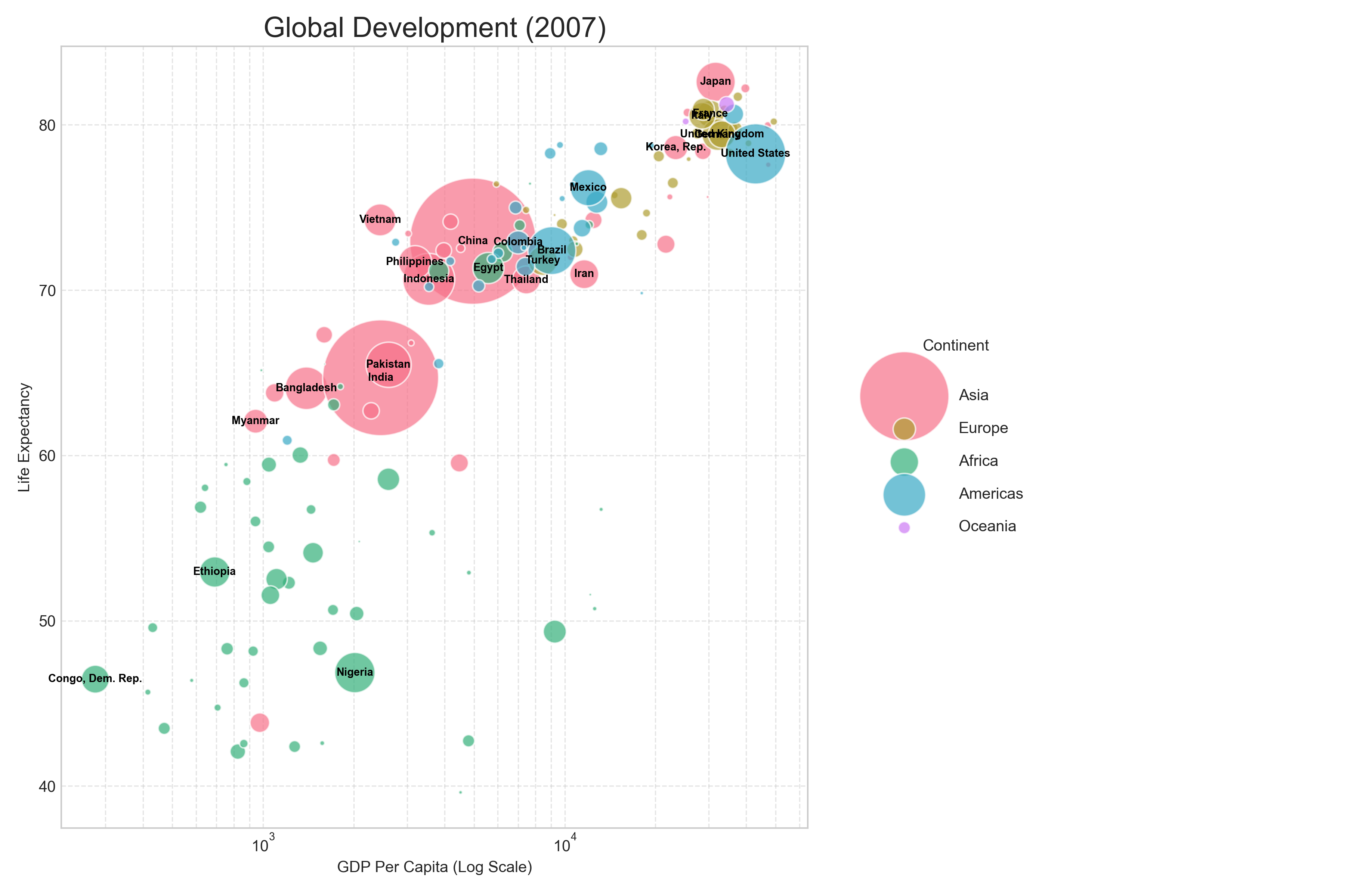
1. The Wealth of Nations (Animated Bubble Chart)
One of the most famous data visualizations is Hans Rosling's bubble chart showing the relationship between GDP per capita and life expectancy over time. Plotly Express allows us to recreate this with an animation slider in just a few lines of code.
import plotly.express as px
import pandas as pd

# Load dataset directly from remote source
url = (
    "https://raw.githubusercontent.com/plotly/datasets/master/gapminderDataFiveYear.csv"
)
gapminder = pd.read_csv(url)

fig = px.scatter(
    gapminder,
    x="gdpPercap",
    y="lifeExp",
    animation_frame="year",
    animation_group="country",
    size="pop",
    color="continent",
    hover_name="country",
    log_x=True,
    size_max=55,
    range_x=[100, 100000],
    range_y=[25, 90],
    title="Global Development (1952-2007)",
)

fig.show()
Interactive Features:
- Play Button: Click play to watch the countries move through time.
- Hover: Hover over any bubble to see the specific country and statistics.
- Legend Filter: Double-click a continent in the legend to isolate it.
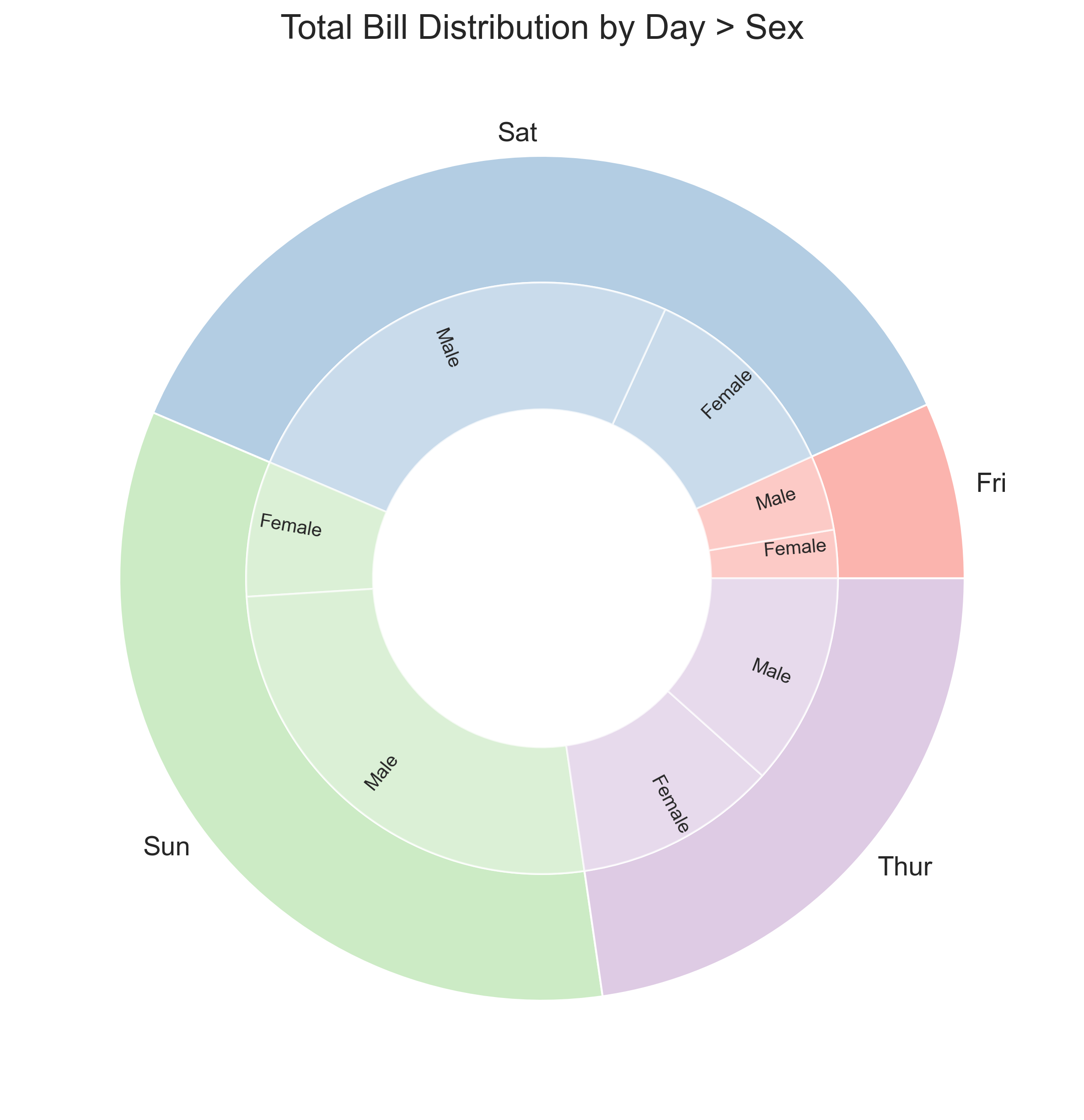
2. Hierarchical Data: Sunburst Charts
Pie charts are often criticized, but Sunburst charts are a powerful way to visualize hierarchical data (like a file system or categorical breakdowns). Here, we visualize the 'Tips' dataset to see how tips are distributed across Days, Times, and Sex.
import plotly.express as px
import pandas as pd

url = "https://raw.githubusercontent.com/plotly/datasets/master/tips.csv"
tips = pd.read_csv(url)

fig = px.sunburst(
    tips,
    path=["day", "time", "sex"],
    values="total_bill",
    color="day",
    title="Total Bill Distribution by Day > Time > Sex",
)
fig.show()
Interactive Features:
- Click to Zoom: Click on "Sun" or "Sat" to zoom in and see the breakdown for just that day. Click the center to zoom back out.
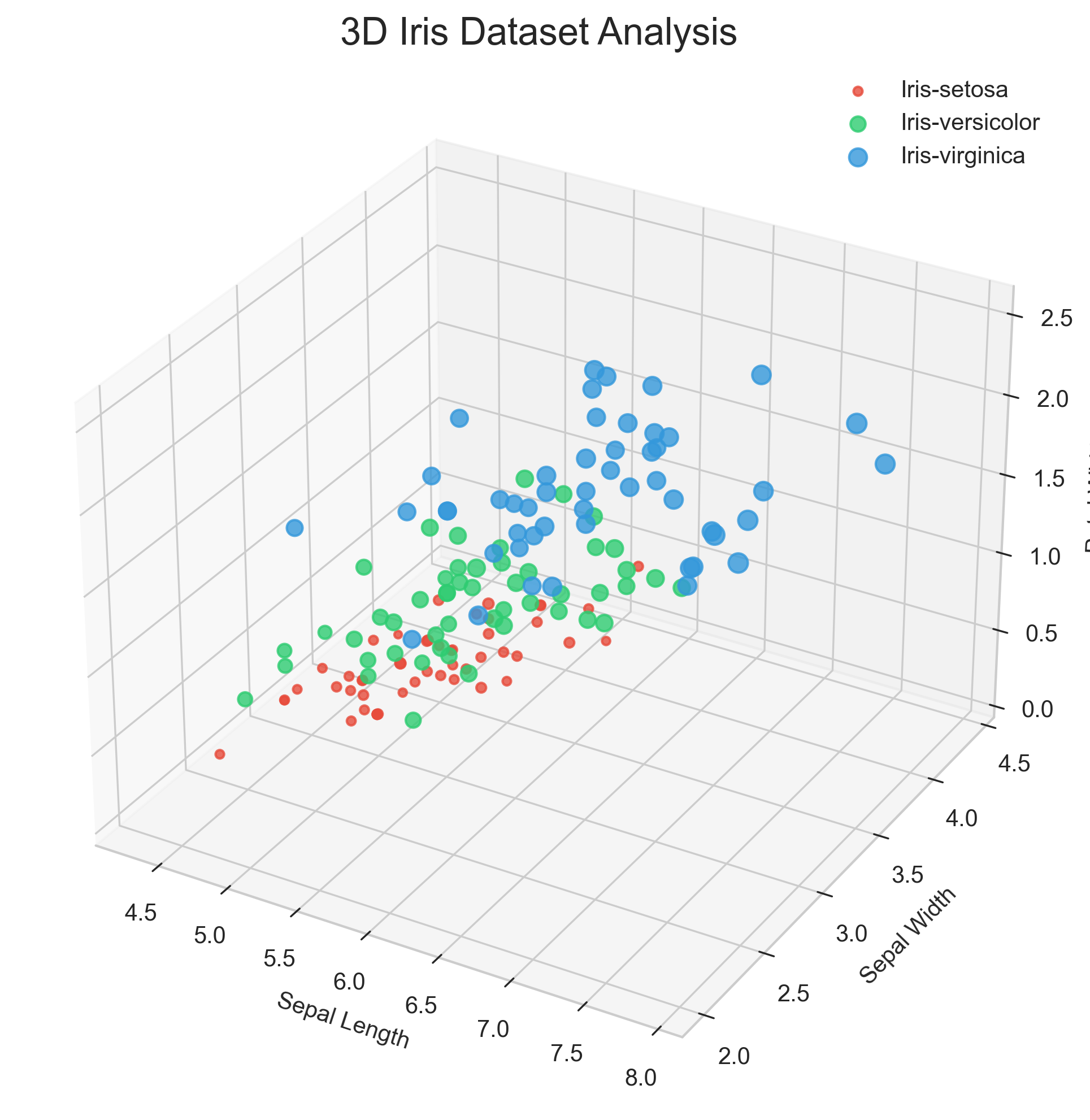
3. 3D Scatter Plots
When you have three continuous variables, a 2D plot can sometimes obscure relationships. A 3D scatter plot allows you to rotate and inspect the data from all angles.
import plotly.express as px
import pandas as pd

url = "https://raw.githubusercontent.com/plotly/datasets/master/iris.csv"
iris = pd.read_csv(url)

fig = px.scatter_3d(
    iris,
    x="SepalLength",
    y="SepalWidth",
    z="PetalWidth",
    color="Name",
    size="PetalLength",
    size_max=18,
    symbol="Name",
    opacity=0.7,
    title="3D Iris Dataset Analysis",
)

fig.update_layout(margin=dict(l=0, r=0, b=0, t=0))
fig.show()
Interactive Features:
- Rotate: Click and drag to rotate the cube.
- Zoom: Scroll to zoom in and out.
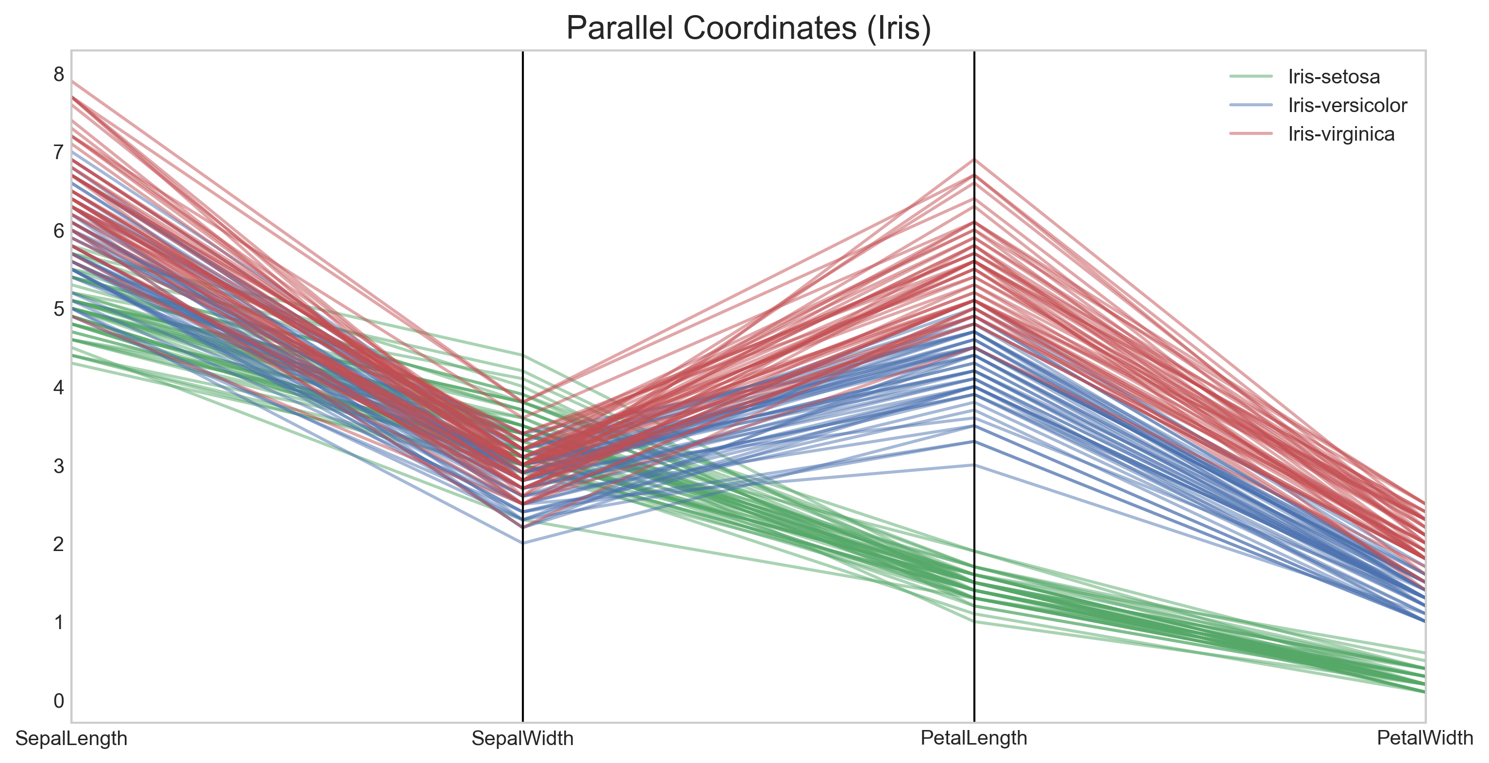
4. Parallel Coordinates
For high-dimensional data (more than 3 dimensions), Parallel Coordinates plots are invaluable. They map each row in the data table as a line passing through parallel axes.
import plotly.express as px
import pandas as pd

url = "https://raw.githubusercontent.com/plotly/datasets/master/iris.csv"
iris = pd.read_csv(url)

# Create numeric ID for color scale
iris["species_id"] = iris["Name"].astype("category").cat.codes

fig = px.parallel_coordinates(
    iris,
    color="species_id",
    labels={
        "species_id": "Species",
        "SepalWidth": "Sepal Width",
        "SepalLength": "Sepal Length",
        "PetalWidth": "Petal Width",
        "PetalLength": "Petal Length",
    },
    color_continuous_scale=px.colors.diverging.Tealrose,
    color_continuous_midpoint=2,
)
fig.show()
Interactive Features:
- Brush Selection: You can drag along any axis to filter lines. For example, select only the high values on the "Petal Length" axis to see which species they correspond to.