Model Deployment
You've preprocessed your data, engineered features, selected an algorithm, and trained a high-performing model. Now what? A model sitting in a notebook is a great academic exercise, but it doesn't provide real-world value until it's deployed.
Model deployment is the process of integrating your machine learning model into an existing production environment where it can take in live data and return predictions. This is the crucial step that bridges the gap between development and operations.
1. Saving and Loading Your Model
Before you can deploy a model, you need to save its trained state (the learned parameters, like the weights and biases). The most common way to do this in Python for standard machine learning models is using the joblib library, which is efficient for saving objects that contain large NumPy arrays.
Saving a trained model:
from sklearn.ensemble import RandomForestClassifier
import joblib

# Assume 'model' is your trained RandomForestClassifier
model = RandomForestClassifier()
# model.fit(X_train, y_train)

# Save the model to a file
joblib.dump(model, "model.joblib")
Loading the model back into memory:
import joblib

# Load the model from the file
loaded_model = joblib.load("model.joblib")

# Use the loaded model to make predictions
# predictions = loaded_model.predict(new_data)
It's also common to use Python's built-in pickle module for this process, as it can serialize any Python object. The syntax is very similar (pickle.dump() and pickle.load()). However, joblib is often preferred for scikit-learn models because it is more efficient at handling the large NumPy arrays that these models contain, which can result in smaller files and faster load times.
For deep learning models, frameworks like TensorFlow and PyTorch have their own built-in functions for saving and loading (e.g., model.save() and tf.keras.models.load_model()).
Common Model Formats
- HDF5 (
.h5): A legacy format for Keras/TensorFlow that saves the entire model (architecture, weights, and optimizer state) in a single file. - TensorFlow SavedModel: The current standard for TensorFlow. Unlike a single file, it's a directory containing a
saved_model.pbfile (the graph) and avariables/subdirectory (the weights), making it highly portable for serving (e.g., via Vertex AI). - PyTorch (
.ptor.pth): Usually stores thestate_dict(weights) or the entire model using Python'spickleformat. - ONNX (
.onnx): The Open Neural Network Exchange format. It's designed for interoperability, allowing you to train in one framework (like PyTorch) and deploy in another. - PMML (
.pmml): Predictive Model Markup Language is an XML-based standard for sharing models between different statistical and data mining tools.
2. Creating a Prediction Service (API)
The most common way to make a model accessible to other applications (like a web front-end or a mobile app) is by wrapping it in an API (Application Programming Interface). You create a simple web server that listens for requests, processes the input data, passes it to your loaded model, and returns the model's prediction in the response.
Flask and FastAPI are two popular Python frameworks for creating simple APIs.
Here is a conceptual example using Flask:
from flask import Flask, request, jsonify
import joblib

# 1. Initialize the Flask app
app = Flask(__name__)

# 2. Load the trained model
model = joblib.load("model.joblib")


# 3. Define a prediction endpoint
@app.route("/predict", methods=["POST"])
def predict():
    # Get the data from the POST request
    data = request.get_json(force=True)

    # Preprocess the data to match the model's input format
    # (e.g., convert to a NumPy array)
    prediction_input = [data["feature1"], data["feature2"]]

    # Make a prediction
    prediction = model.predict([prediction_input])

    # Return the prediction as a JSON response
    return jsonify({"prediction": int(prediction[0])})


# 4. Run the app
if __name__ == "__main__":
    app.run(port=5000, debug=True)
You could then send a request to this running server and get a prediction back, effectively making your model a usable service.
3. Deployment Environments
Once you have your model wrapped in an API, you need to host it somewhere.
- On-Premise Servers: Traditional deployment on your own company's servers.
- Cloud Platforms (IaaS/PaaS): You can run your API on a virtual machine (like an AWS EC2 instance) or a platform-as-a-service (like Heroku).
- Managed ML Services (Serverless): Cloud providers offer services specifically for deploying models, which handle the underlying infrastructure for you. This is often the most scalable and efficient approach. Examples include:
- AWS SageMaker Endpoints
- Vertex AI (Google Cloud)
- Azure Machine Learning
4. Production Deployment with Vertex AI
For production-ready applications, Vertex AI on Google Cloud simplifies the deployment process by providing managed infrastructure:
- Model Registry: Acts as a central repository to store, version, and manage your machine learning models.
- Endpoints: Models are deployed to Endpoints for real-time (online) predictions. Vertex AI manages the underlying compute resources and provides a REST API.
- Autoscaling: Automatically adjusts the number of nodes serving your model based on incoming traffic to ensure performance and cost-efficiency.
- Traffic Splitting: Allows you to route a portion of traffic to different model versions (e.g., for A/B testing or canary releases).
- Batch Prediction: For large datasets that don't require immediate responses, you can run batch jobs to process data in bulk.
Multi-Model Endpoints and Traffic Splitting
In Vertex AI, you can deploy more than one model to the same endpoint. This is a powerful feature for managing updates without disrupting your live application.
Reasons to deploy multiple models to one endpoint:
- Gradual Rollouts (Canary Deployment): When you have a new version of a model (e.g., trained on newer data or with better accuracy), you can deploy it to the existing endpoint alongside the old version. By assigning a small percentage of traffic (e.g., 5%) to the new model, you can test its performance in the real world before committing fully.
- Stable API URLs: Your client application (web or mobile) points to a single endpoint URL. By using multi-model deployment, you can swap models or change traffic splits entirely on the backend without ever needing to update the code in your front-end application.
- Safe Promotion: You can gradually increase the traffic split (5% -> 20% -> 50% -> 100%) as you gain confidence in the new model's performance.
Best Practice: While Vertex AI allows you to deploy models of different types (e.g., one AutoML and one Custom-trained) to the same endpoint because resources are associated with the model itself, the best practice is to deploy models of a specific type to an endpoint. This makes the environment much easier to manage, monitor, and troubleshoot.
💡 Managed Endpoints vs. Physical Ports In a local environment (like Flask), you cannot have two models "listening" on the same port (e.g.,
:5000). However, in the cloud, an Endpoint is a logical router. When you deploy multiple models to one endpoint, each model runs on its own isolated compute resources (different VMs or containers). The Endpoint acts as a load balancer, receiving requests at a single stable URL and forwarding them to the appropriate model based on your traffic split settings.
5. Model Monitoring
Deployment is not the final step. Once a model is in production, its performance can degrade over time due to changes in the real-world data it receives. This is known as model drift or concept drift.
It's crucial to monitor your deployed model for:
- Performance Metrics: Is the accuracy (or other key metrics) of the model's predictions staying consistent?
- Data Drift: Is the statistical distribution of the live data significantly different from the data the model was trained on?
Skew vs. Drift
| Feature | Skew | Drift |
|---|---|---|
| Comparison | Training Data vs. Serving Data | Serving Data (Today) vs. Serving Data (Last Month) |
| Timing | Immediate (as soon as you deploy) | Gradual (happens over weeks or months) |
| Cause | Data pipeline errors, different data sources, or poor sampling. | Changes in the real world, consumer behavior, or environment. |
| Detection | Vertex AI Model Monitoring (Training-Serving Skew) | Vertex AI Model Monitoring (Prediction/Feature Drift) |
Model Monitoring Metrics (Vertex AI)
To detect skew and drift, production systems use specific statistical distance metrics to compare the baseline (Training) to the latest data (Serving).
| Monitoring Type | Description | Feature Types | Metric |
|---|---|---|---|
| Input Feature Drift | Measures distribution of input feature values compared to baseline. | Categorical | L-Infinity, Jensen Shannon Divergence |
| Numerical | Jensen Shannon Divergence | ||
| Output Inference Drift | Measures model's predictions distribution compared to baseline. | Categorical | L-Infinity, Jensen Shannon Divergence |
| Numerical | Jensen Shannon Divergence | ||
| Feature Attribution | Measures the change in contribution of features to a model's inference. | Numerical/Categorical | Feature Importance Shift |
What is Feature Attribution Monitoring?
Unlike data drift (which looks at inputs) or inference drift (which looks at outputs), Feature Attribution tracks if the importance of a feature has changed.
For example, if your housing model originally relied heavily on "Square Footage" to make predictions, but suddenly "Zip Code" becomes the dominant factor in production, the model's internal logic has shifted. This can indicate that the underlying relationship between features and the target has changed, even if the distributions of individual features look normal.
Examples in Practice
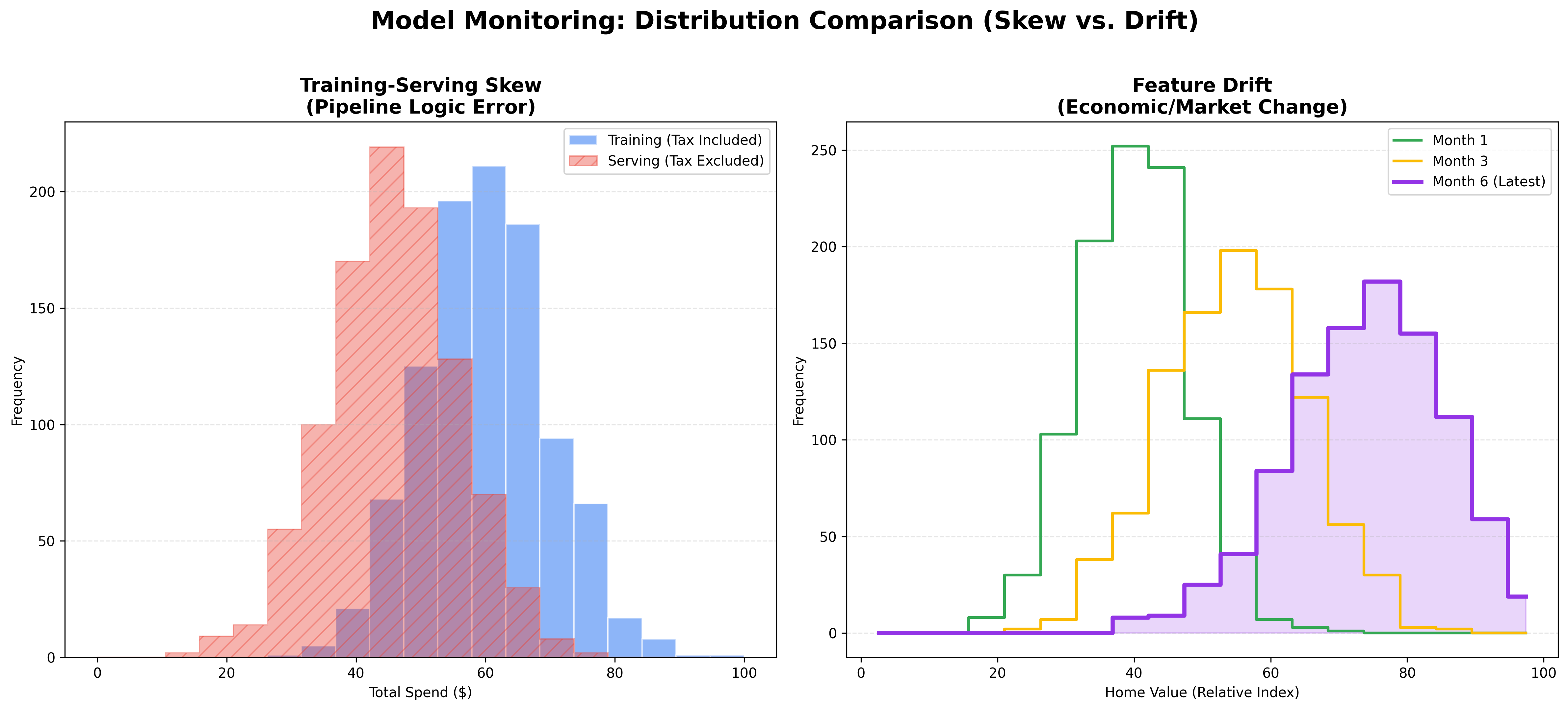
- Skew Example (Pipeline Error): A churn prediction model is trained on a database where "Total Spend" includes tax. However, the live API serving the model provides "Total Spend" excluding tax. The model immediately sees lower spend values than expected (shifting the serving distribution to the left of the baseline), leading to incorrect churn predictions from day one.
- Drift Example (Environmental Change): A housing price model is deployed in a city where a new major tech hub suddenly opens. Over several months, as demand spikes, the average "Home Value" distribution drifts significantly to the right (higher prices) compared to the original training data. By "Month 6," the model's original price relationships are no longer accurate due to this market shift.
If performance degrades, it's a signal that the model needs to be retrained on new, more recent data.
Operational Guidelines for Model Quality
Beyond monitoring for drift, maintaining a high-quality ML solution requires adhering to rigorous operational best practices throughout the model lifecycle. According to Google Cloud's Guidelines for Model Quality, teams should implement the following technical checks:
1. Verify Basic Learning Ability
- The "Tiny Dataset" Test: Before full-scale training, ensure your model doesn't have fundamental bugs by training it on just a few examples. If the model cannot achieve near-perfect accuracy on this tiny subset (overfitting it intentionally), there is likely a bug in your model architecture or training routine.
2. Detect Numerical Instability
- Monitor for NaN Values: Always track the training and serving logs for
NaN(Not a Number) values in the loss function. This is often a sign of erroneous arithmetic calculations, exploding gradients, or division by zero. - Track Zero-Valued Weights: Monitor the percentage of weights that are exactly zero. High percentages can indicate vanishing gradients or overly aggressive regularization.
- Visualize Internal Shifts: Periodically visualize weight-value distributions over time. Detecting Internal Covariate Shift early allows you to apply corrective measures like Batch Normalization to restore training speed.
3. Deep-Dive Performance Analysis
- Compare Train vs. Test: Regularly compare performance on training vs. test data to detect Underfitting (increase learning capacity) or Overfitting (apply regularization).
- High-Confidence Error Analysis: Don't just look at aggregate metrics. Analyze instances where the model makes a wrong prediction with high confidence. This often reveals mislabeled training data or extreme outliers.
- Confusion Matrix Deep-Dives: In multi-class problems, identify the "most-confused classes." These patterns indicate where you might need better data preprocessing or new features to help the model discriminate between similar categories.
4. Model Parsimony (Simplicity)
- Feature Selection: Analyze feature importance scores and aggressively remove features that do not provide significant quality improvements. Parsimonious models (simpler models) are always preferred over complex ones as they are easier to maintain, faster to serve, and less prone to unexpected behavior.
(Guidelines adapted from Google Cloud Architecture Framework: Model Quality.)
Guidelines for Production Monitoring
Once a model is deployed, continuous monitoring is essential to ensure it remains reliable and efficient. According to Google Cloud's Guidelines for Production Monitoring, teams should implement the following:
1. Data Logging and Profiling
- Request-Response Logging: Log a sample of serving payloads (input data and model predictions) for regular analysis.
- Automated Profiling: Implement processes to compute descriptive statistics on serving data at regular intervals to detect changes in data patterns.
2. Drift and Outlier Detection
- Training-Serving Skew: Compare serving data statistics to the training baseline to identify immediate skews or gradual drift.
- Feature Attribution Tracking: Monitor how much each feature contributes to predictions over time. Changes here often signal Concept Drift (the relationship between inputs and outputs has changed).
- Outlier Identification: Use novelty detection to find serving instances that are significantly different from training data. Track the percentage of these outliers over time.
3. Continuous Evaluation and Alerts
- Threshold Alerts: Set automated alerts for when skew scores on key predictive features cross defined limits.
- Ground Truth Joins: If actual outcomes (ground truth) become available later, join them with your predictions to perform Continuous Evaluation. This identifies specifically which types of requests the model handles well or poorly.
4. System Efficiency
- Performance Objectives: Set clear objectives for system metrics (e.g., latency, throughput) and measure your model against them.
- Resource Monitoring: Track CPU, GPU, and memory utilization, along with service latency and error rates, to manage capacity and estimate infrastructure costs.
(Guidelines adapted from Google Cloud Architecture Framework: Production Monitoring.)