Convolutional Neural Networks (CNNs)

When it comes to tasks involving images and spatial data, such as image classification, object detection, and image segmentation, Convolutional Neural Networks (CNNs or ConvNets) are the gold standard. Unlike Multilayer Perceptrons (MLPs), which treat inputs as flat vectors, CNNs are designed to respect and exploit the 2D structure of images.

The Problem with MLPs for Images

A moderately sized color image can have millions of pixels. If you were to flatten this image into a vector and feed it into an MLP, the number of parameters in the first hidden layer would be enormous. For example, a 1000x1000 pixel image fed into a hidden layer with just 100 neurons would result in hundreds of millions of weights. This makes the model incredibly slow to train, memory-intensive, and highly prone to overfitting.

CNNs solve this problem by using two key principles: locality and translation invariance.

Locality: The network assumes that pixels that are close to each other are more strongly related than pixels that are far apart.
Translation Invariance: The network assumes that if a pattern (like a cat's ear) is important in one part of the image, it will be important in any other part of the image.

CNN Architecture

The Core Component: The Convolutional Layer

Instead of connecting every input pixel to every neuron, a CNN uses convolutional layers that apply a small filter (or kernel) across the entire image.

Convolution Operation

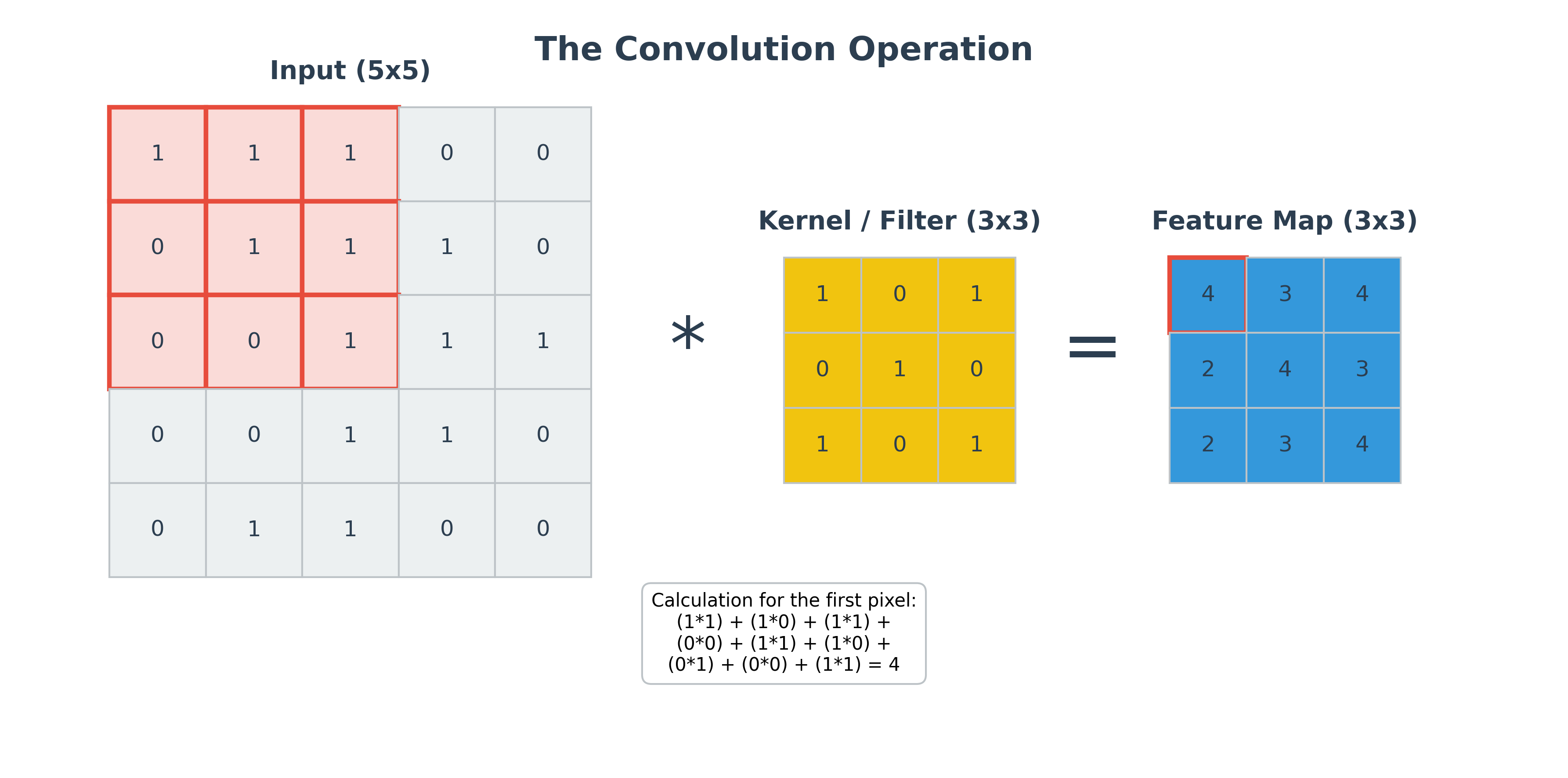
This kernel is a small matrix of learnable weights. It slides over the input image, and at each position, it computes the dot product between the kernel and the patch of the image it is currently on. This process produces a feature map, which highlights the presence of the specific feature the kernel is looking for (e.g., a vertical edge, a specific color, a texture).

Because the same kernel is used across the entire image, the number of parameters is drastically reduced. The network learns the weights of the kernel, effectively learning what features are important to look for.

Padding and Stride

Padding: Convolution operations tend to shrink the output feature map. To maintain the spatial dimensions, we can add a border of zeros around the input image. This is called padding.
Stride: The stride is the number of pixels the kernel moves at each step. A stride of 1 moves the kernel one pixel at a time. A larger stride will result in a smaller output feature map, effectively downsampling the image.

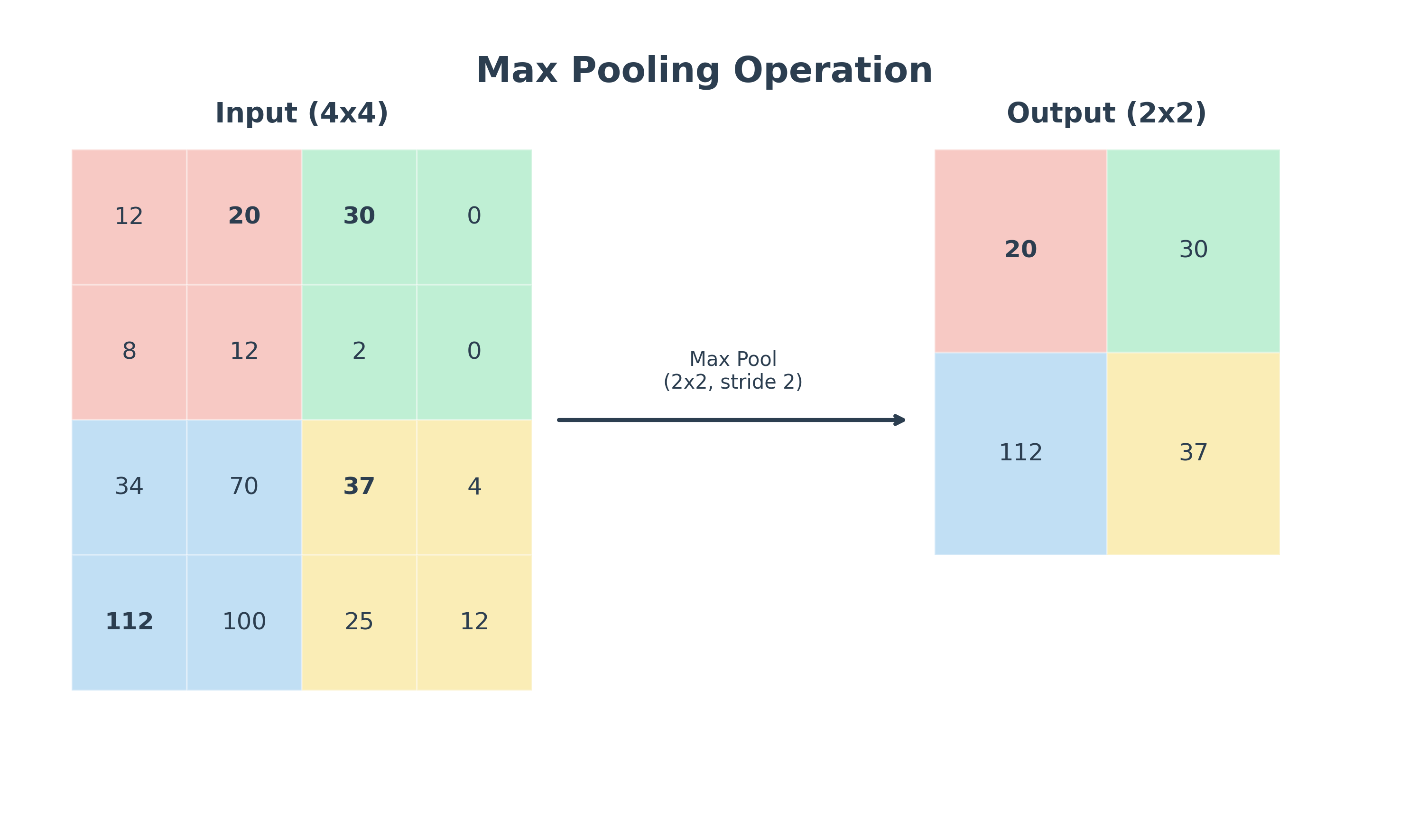
Pooling Layers: Downsampling

After a convolutional layer, it is common to add a pooling layer. The purpose of a pooling layer is to reduce the spatial dimensions (width and height) of the feature map, which has several benefits:

It reduces the number of parameters and computation in the network.
It makes the feature representations more robust to small translations in the input image.

The most common type of pooling is Max Pooling. It works by sliding a window over the feature map and, for each window, taking the maximum value.

Max Pooling

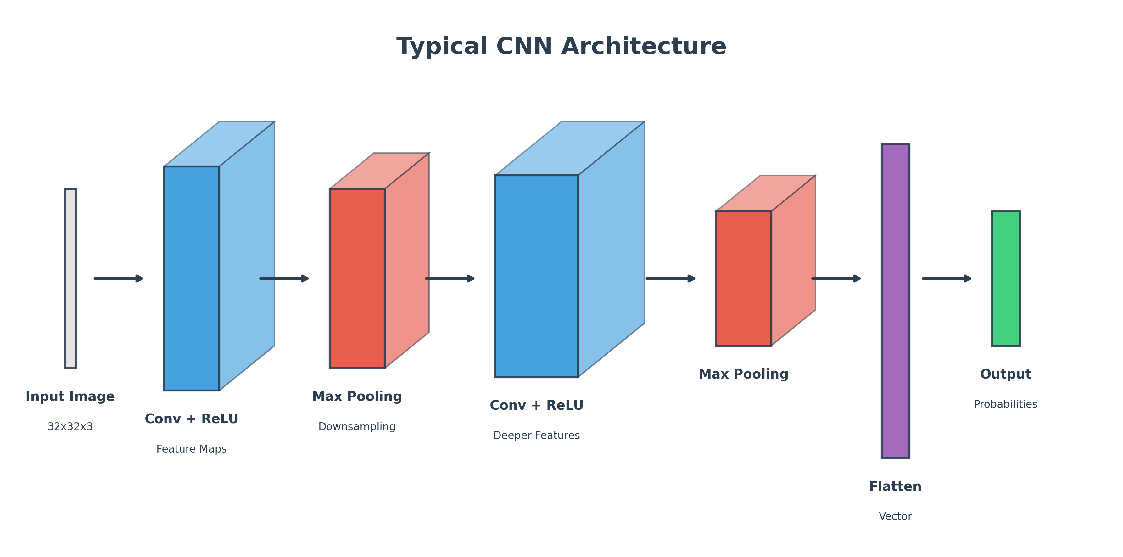
Building a CNN in PyTorch

A typical CNN architecture consists of a stack of convolutional layers and pooling layers, followed by one or more fully-connected (MLP) layers at the end to perform the final classification.

Here is a simplified example of a CNN for image classification in PyTorch:

import torch.nn as nn
import torch.nn.functional as F


class SimpleCNN(nn.Module):
    def __init__(self):
        super().__init__()
        # First convolutional layer
        self.conv1 = nn.Conv2d(in_channels=3, out_channels=16, kernel_size=3, padding=1)
        # Second convolutional layer
        self.conv2 = nn.Conv2d(
            in_channels=16, out_channels=32, kernel_size=3, padding=1
        )
        # Max pooling layer
        self.pool = nn.MaxPool2d(kernel_size=2, stride=2)
        # Fully connected layers
        self.fc1 = nn.Linear(32 * 8 * 8, 256)  # Assuming 32x32 input image
        self.fc2 = nn.Linear(256, 10)  # 10 output classes

    def forward(self, x):
        # Apply convolutions, activation functions, and pooling
        x = self.pool(F.relu(self.conv1(x)))
        x = self.pool(F.relu(self.conv2(x)))

        # Flatten the image for the fully connected layers
        x = x.view(-1, 32 * 8 * 8)

        # Apply fully connected layers
        x = F.relu(self.fc1(x))
        x = self.fc2(x)
        return x

This structure of stacking convolutional and pooling layers is the foundation of most modern computer vision architectures.

Transfer Learning: Standing on the Shoulders of Giants

Training a state-of-the-art CNN from scratch requires millions of labeled images and massive computational power (GPUs). Transfer Learning is a technique where you take a model trained on a very large dataset (like ImageNet, which has 1.4 million images) and repurpose it for your specific, smaller task.

Transfer Learning Comparison

This is highly efficient because the early layers of a CNN learn generic features like edges, textures, and shapes that are useful for any image task.

The Two Main Strategies

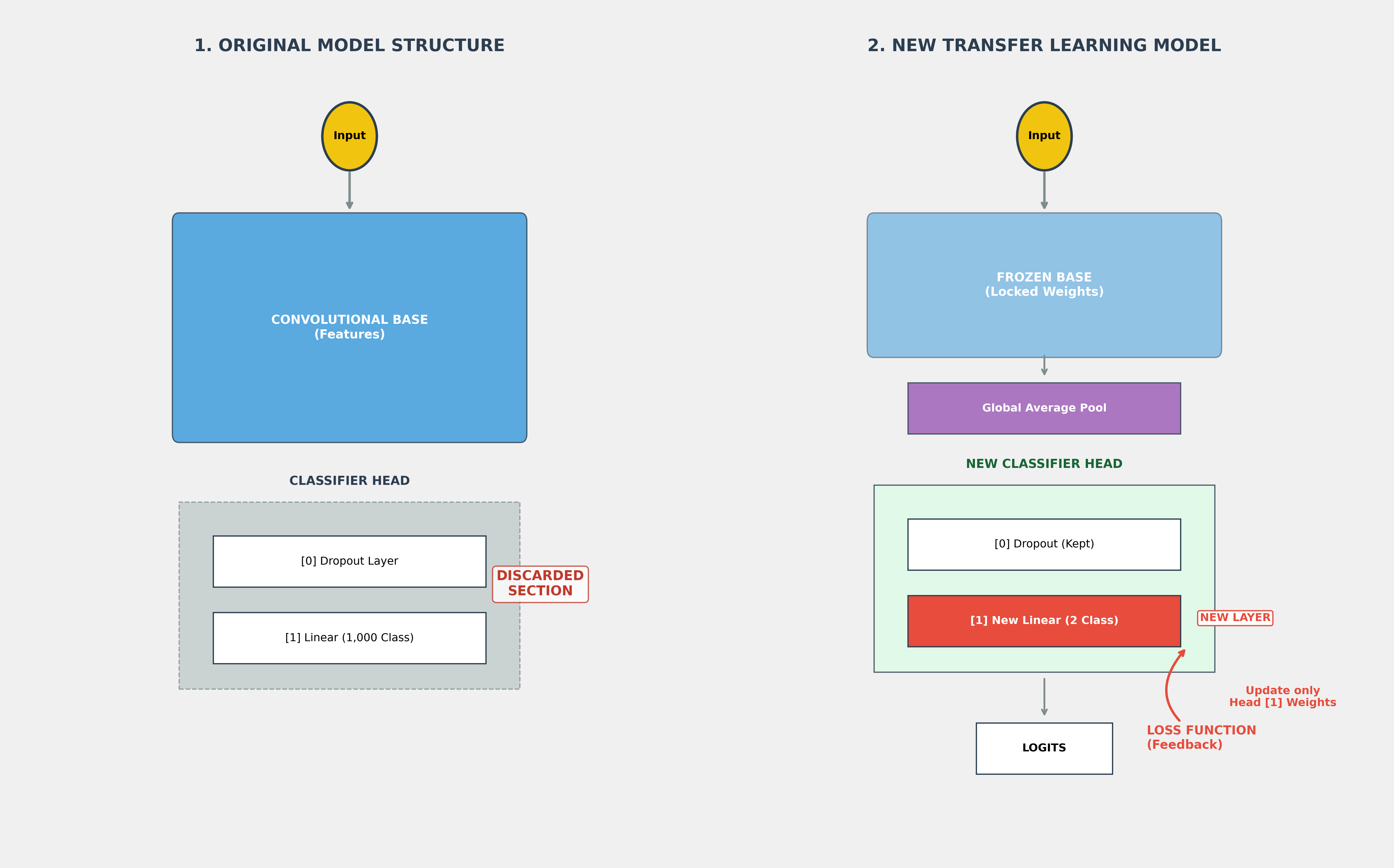
Feature Extraction (Freezing the Base):
- You take a pre-trained model (e.g., MobileNet V2, ResNet, or VGG).
- You "freeze" all the convolutional layers so their weights don't change.
- You replace the final classification "head" with a new one suited for your classes (e.g., "Cats vs. Dogs").
- Only the new head is trained. This is perfect for very small datasets.
Fine-Tuning:
- After training the new head, you "unfreeze" a few of the top convolutional layers.
- You train the entire model again with a very low learning rate.
- This allows the model to "fine-tune" the higher-level features to better fit your specific data.

Example: Transfer Learning in PyTorch

Using a pre-trained model like MobileNet V2 is straightforward:

import torch
import torchvision.models as models
import torch.nn as nn

# 1. Load a pre-trained model (e.g., MobileNet V2)
model = models.mobilenet_v2(pretrained=True)

# 2. Freeze all parameters in the base model
for param in model.parameters():
    param.requires_grad = False

# 3. Replace the final classification head
# model.classifier is a Sequential block: [0] is Dropout, [1] is the Linear head
num_features = model.classifier[1].in_features
model.classifier[1] = nn.Linear(
    num_features, 2
)  # Replace the 1000-class head with a 2-class head

# 4. Now only the weights of the new Linear layer will be updated
optimizer = torch.optim.Adam(model.classifier[1].parameters(), lr=0.001)

Example: Transfer Learning in TensorFlow/Keras

As seen in the official TensorFlow Transfer Learning Tutorial, the implementation in Keras is highly declarative and concise:

import tensorflow as tf

# 1. Load the pre-trained MobileNet V2 model
# include_top=False removes the final classification layer
# This automatically resizes any image (large or small) to 160x160
base_model = tf.keras.applications.MobileNetV2(
    input_shape=(160, 160, 3), include_top=False, weights="imagenet"
)

# 2. Freeze the convolutional base
base_model.trainable = False

# 3. Build the new model with a classification head
model = tf.keras.Sequential(
    [
        base_model,
        tf.keras.layers.GlobalAveragePooling2D(),
        tf.keras.layers.Dense(2),  # New head for 2 classes (e.g., Cats vs Dogs)
    ]
)

# 4. Compile and train (only the Dense layer weights will update)
model.compile(
    optimizer=tf.keras.optimizers.Adam(learning_rate=0.0001),
    loss=tf.keras.losses.BinaryCrossentropy(from_logits=True),
    metrics=["accuracy"],
)

Key Components Explained

input_shape=(160, 160, 3): This defines the resolution and color format of the input images. 160x160 is the pixel resolution (Height x Width), and 3 represents the RGB color channels.
Image Resizing (Preprocessing): While your raw image files (JPG/PNG) can be any size, they must be resized to exactly 160x160 before entering the model. This is handled automatically by preprocessing layers (like image_dataset_from_directory), which ensures all images in a "batch" have the same dimensions for GPU processing.
include_top=False: This is critical. It tells Keras not to load the original 1,000-class classification layer of MobileNetV2. We replace this "top" with our own custom head for our specific task (e.g., 2 classes for Cats vs. Dogs).
weights='imagenet': This loads the specific, pre-calculated weights from the model's original training on the massive ImageNet dataset. Without this, the model would start with random weights and require much more data to train.
base_model.trainable = False (Freezing): This "freezes" the convolutional layers. We want to keep the knowledge (edges, textures) the model already has. If we didn't freeze them, the initial training of our new head would destroy these valuable pre-learned features.
GlobalAveragePooling2D(): This layer converts the 3D block of features (spatial data) into a 1D vector. Although the input is 3D (Height $\times$ Width $\times$ Channels), it is called 2D because it calculates the average across the two spatial dimensions (Height and Width) for each channel independently. This drastically reduces the number of parameters and makes the model more efficient and less prone to overfitting compared to a Flatten() layer.
Dense(2): This is our new classification head. Each neuron represents one of our target classes. It produces raw numbers called logits.
from_logits=True: In the loss function, this indicates that the model's output is raw logits that haven't been "squashed" into probabilities yet. Calculating loss directly from logits is numerically more stable during training.